michalkokta

Alexander Zverev vs. Rafael Nadal: A Tale of Two Matches

En route to his recent ATP Masters 1000 title in Madrid, Alexander Zverev notched his first clay court victory over Rafael Nadal. Zverev beat Nadal twice before their Madrid encounter, but both victories came on indoor hard courts. Playing Nadal on clay is a different animal though. His confidence on clay is sky high, the higher bounces magnify Nadal’s ability to hit the ball with heavy topspin, and the slower conditions tend to make matches more physical, which Nadal relishes.

After Zverev took the match 6-4 6-4 in the quarter finals in Madrid, the two were set for a rematch a week later in the quarter finals of the ATP Masters 1000 in Rome. This time it was Nadal, who came away with the 6-3 6-4 victory. Looking at the statistics from both matches, we can catch a glimpse of the adjustments that Nadal made, and how he was able to tilt the way the match was played in his favor in Rome more so than in Madrid.

Extending the Points

Let’s first take a look at the distribution of the different rally lengths from the Madrid match, which Zverev won.

	Total Points	Percent of Total	Zverev	Nadal	Advantage
0-4 shots	65	59.63%	36	29	Zverev +7
5-8 shots	29	26.61%	18	11	Zverev +7
9+ shots	15	13.76%	6	9	Nadal +3

Courtesy ATPTour.com

Almost 60% of the points in Madrid were shorter than 4 shots, and over 85% were shorter than 8 shots. The average rally length for the match was 5.9 shots. It was in these shorter rallies where Zverev won the match. Once the rally extended past 9 shots, it was advantage Nadal; but since those rallies counted for less than 15% of all points, it was not enough to swing the match in Nadal’s favor.

Going into the match in Rome, I would assume that one of Nadal’s goals was to work his way into the point, extend the rallies, and make the match more physical than was the case in Madrid. Let’s examine the same statistics from Rome.

	Total Points	Percent of Total	Zverev	Nadal	Advantage
0-4 shots	44	34.92%	25	19	Zverev +6
5-8 shots	50	39.68%	22	28	Nadal +6
9+ shots	32	25.40%	12	20	Nadal +8

Courtesy ATPTour.com

Mission accomplished for Nadal. Zverev still won the 0-4 shot rally length, but the percentage of total points in that particular bucket dropped from about 60% in Madrid to only about 35% in Rome. Conversely, the contribution of the 9+ rally length increased from about 14% in Madrid to over 25% in Rome. Combine those two, and the average rally length in Rome jumped to 7.5 shots compared to the 5.9 average in Madrid. Furthermore, Nadal was able to reverse the 5-8 shot rally length to his advantage, and maintain his dominance in the extended 9+ shot rallies.

How exactly was Nadal able to extend the rallies in Rome compared to Madrid? By going into Zverev’s backhand more, and by hitting spinnier, heavier groundstrokes.

Targeting the Zverev Backhand

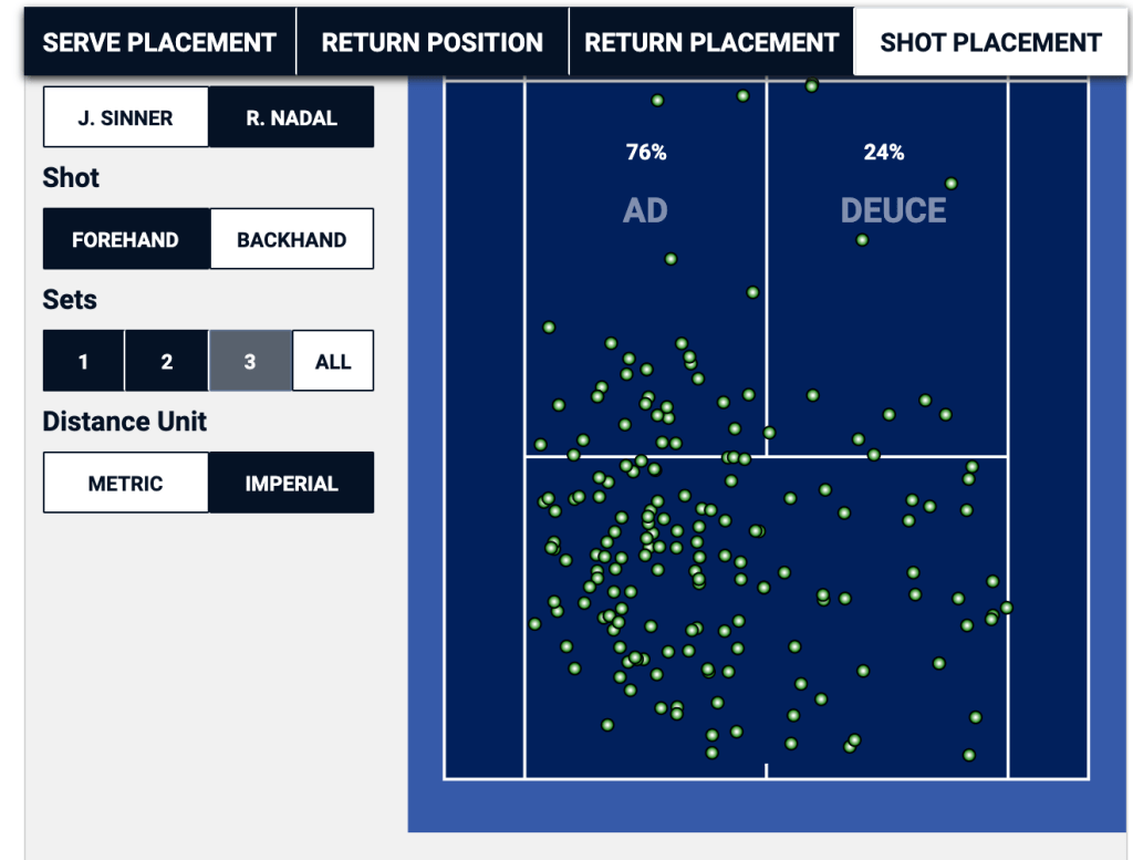
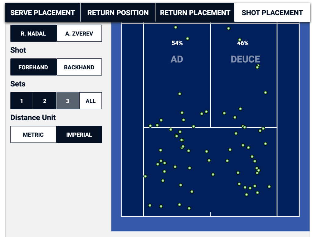
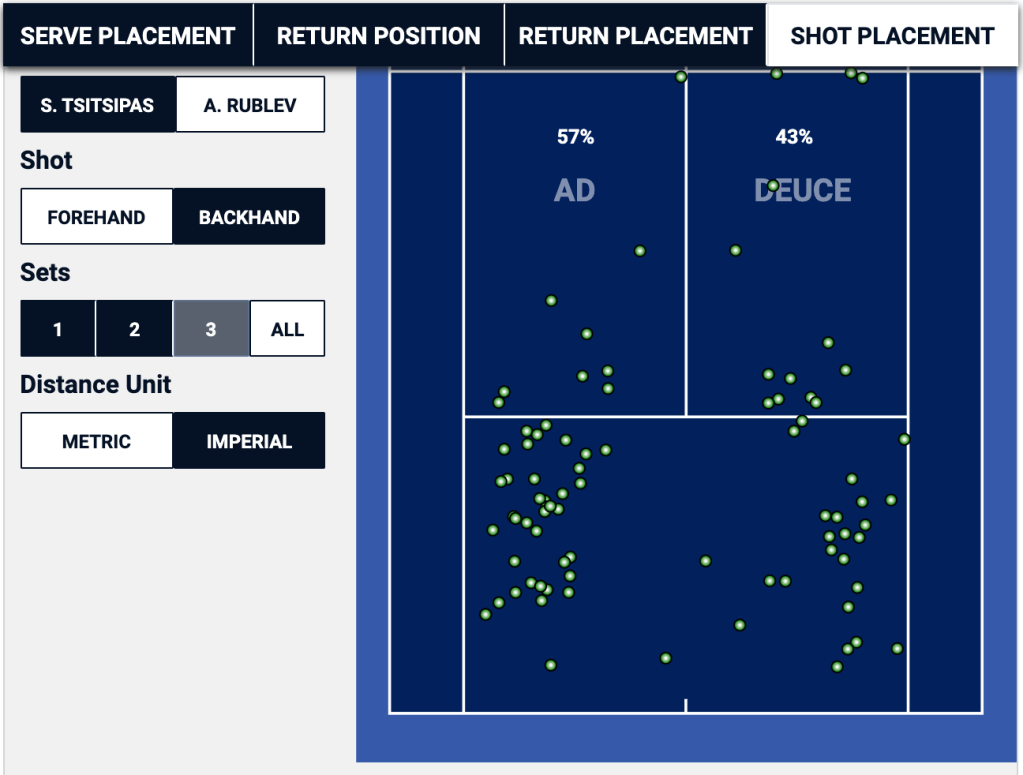
Once the point got started, Nadal’s strategy in Rome was much more focused on hitting through the Zverev backhand than was the case in Madrid. Let’s look first at the comparison of Nadal’s forehand targets from both matches:

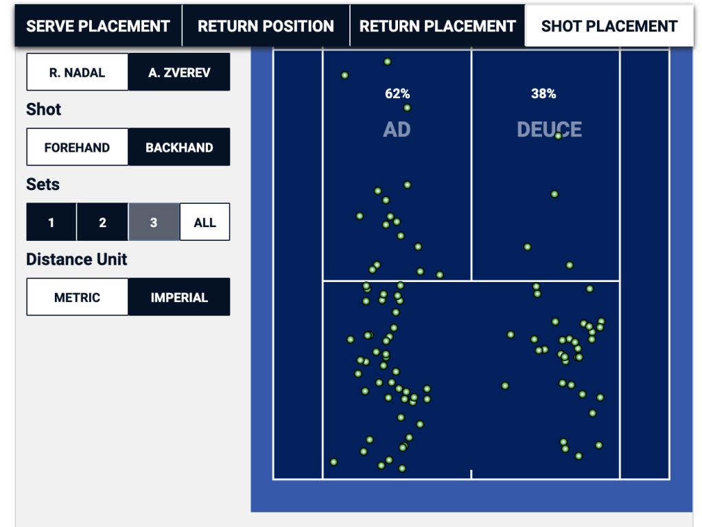
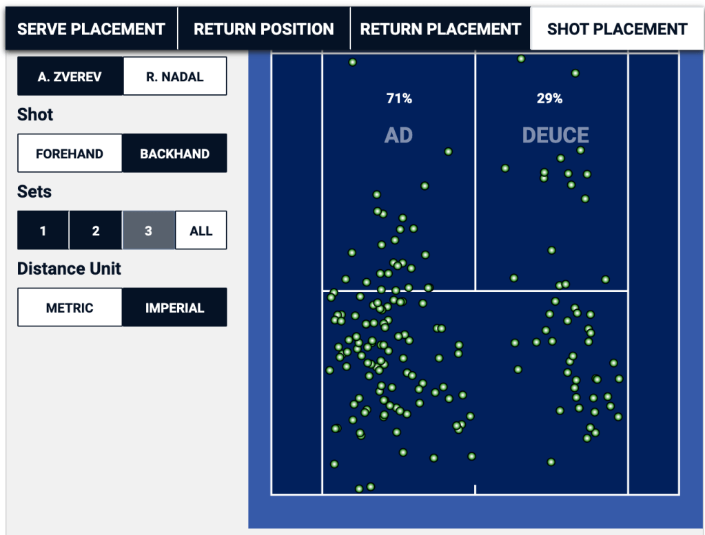
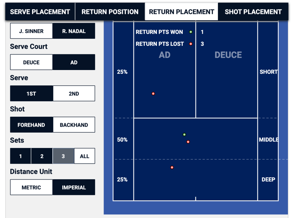
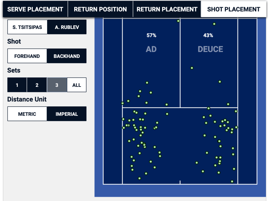
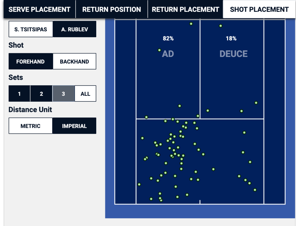
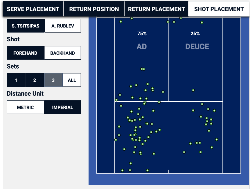
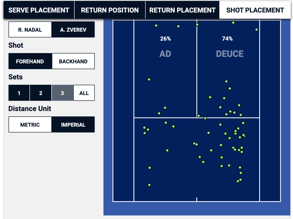
The left image are Nadal’s forehands in Madrid, where he lost, and the image on the right is Nadal’s forehands in Rome, where he won. There is about a 10% increase in Nadal’s forehands being aimed cross-court into Zverev’s backhand. The difference is yet more pronounced on Nadal’s backhands:

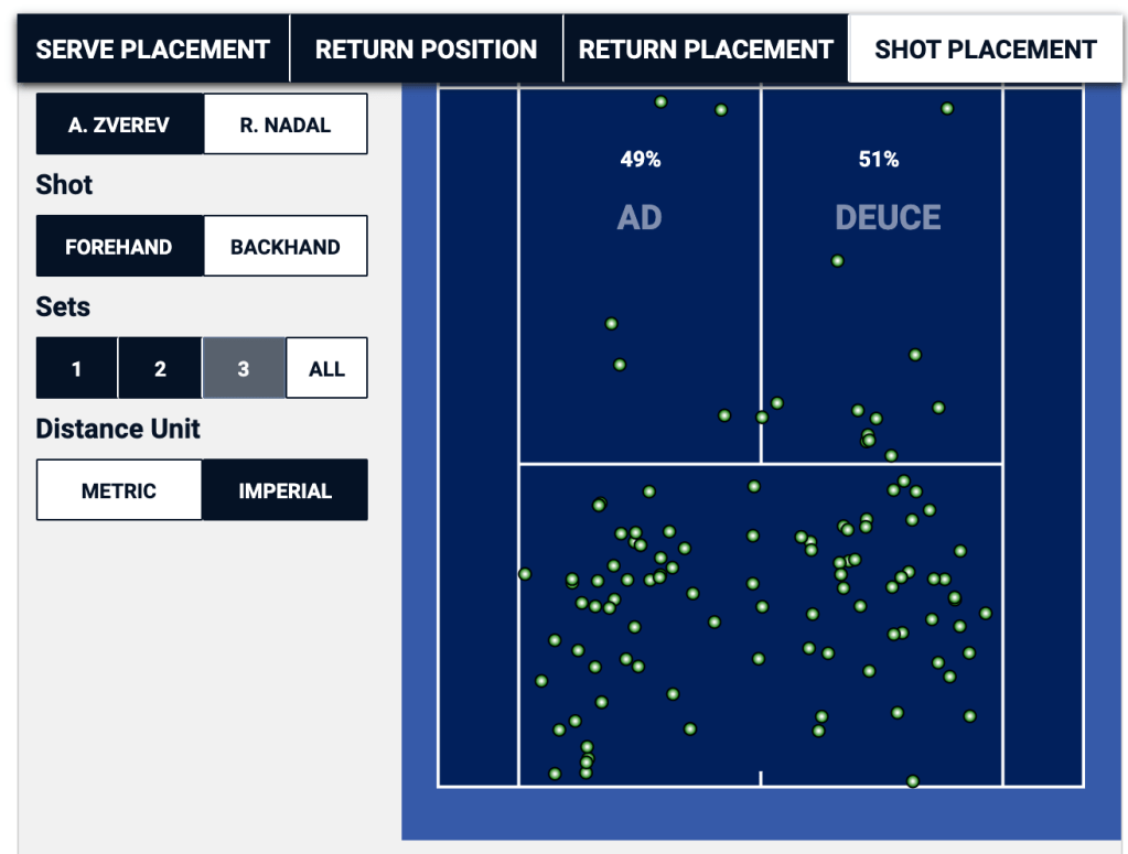
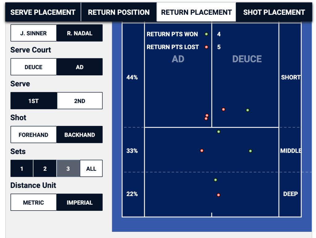
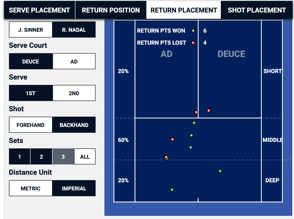
The left image is once again Nadal’s backhands from Madrid. In that match, Nadal hit 3 out of every 4 backhand cross-court into Zverev’s forehand. In Rome, Nadal made sure to stay away from that particular pattern more often, and his backhands were split about evenly between cross-court and down the line. Also, notice the higher frequency with which Nadal’s backhands were landing deeper in the court in Rome than was the case in Madrid. Depth is one of the best ways to gain control of the point in a rally, and it was surely a contributing factor in Zverev committing 31 rally unforced errors in Rome as compared to just 10 in Madrid.

Heavier Spin on Groundstrokes

Not only did Nadal get his groundstrokes – especially backhands – deeper into the court in Rome, his strokes were also “heavier,” hit with more topspin. Below is a table comparing the average RPMs on groundstrokes from both the Madrid and the Rome matches.

	Nadal FH	Nadal BH	Zverev FH	Zverev BH
Madrid	3,069 rpm	2,378 rpm	2,893 rpm	1,529 rpm
Rome	3,183 rpm	2,578 rpm	2,830 rpm	1,500 rpm
Difference	+114 rpm	+200 rpm	-63 rpm	-29 rpm

Courtesy ATPTour.com

While Zverev was hitting his groundstrokes flatter in Rome than he did in Madrid, Nadal really cranked up the topspin, especially on his backhand wing. Knowing that balls with more topspin tend to bounce higher than flatter strokes, and combining that with the groundstroke distribution patterns, we can try to guess Nadal’s baseline strategy in Rome: try to get the ball up high on Zverev’s backhand, making it harder for him to attack from that part of the court. Now, Alexander Zverev is listed at 6’6″, so this is no easy feat.

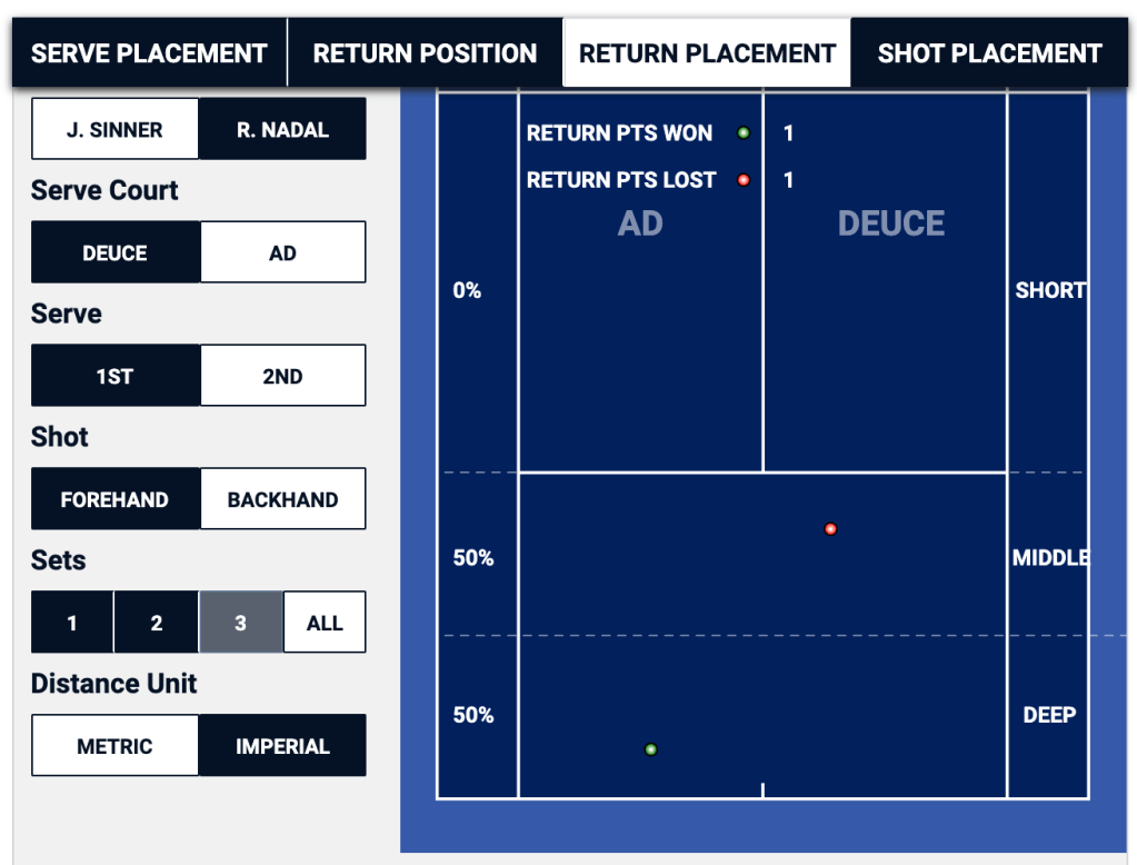
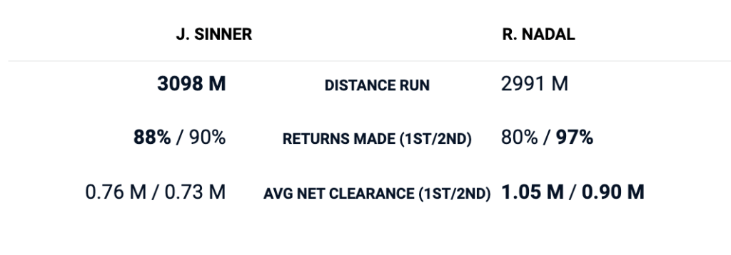
It would be great to see the average net clearance of Nadal’s groundstrokes in the match, but I can’t seem to find that statistic on the ATP website. The best I can do is compare the average net clearance on Nadal’s second serve returns, which were hit about 0.81m above the net in Madrid, and about 20cm higher – 1.03m above the net – in Rome. It is certainly not hard evidence, but it points in the same general direction as the higher rpms on the groundstrokes: get the ball higher on Zverev.

Getting the ball deep and under heavy spin into Zverev’s backhand forces Zverev into a decision. Option one is to try to take the ball on the rise, before it gets up above his shoulders. The timing of that shot is tricky even for the best players in our sport, and given how flat Zverev’s backhand is, the margin for error is slim. Alternatively, Zverev can back up and wait until the ball drops back down into his strike zone. That, however, puts him in a defensive position way behind the baseline – minimizing his chance to attack – most likely extending the rally – and playing right into Nadal’s hands. Pick your poison time for Zverev.

Alexander Zverev was able to get the best out of Rafael Nadal in Madrid by keeping the majority of the rallies short. Nadal countered in Rome with a strategy designed to extend the rallies, and trying to get Zverev uncomfortable in the ad side of the court. Should these two face-off at the French Open, one of the factors deciding the outcome of the match will be the length of the rallies. If Zverev can keep the match a first-strike battle, he has a chance. Otherwise, with every extra groundstroke hit, Nadal’s advantage will keep mounting.

3 Suggestions for Jannik Sinner Against Rafael Nadal

After losing to Rafael Nadal in the 2nd round of the ATP Rome Masters 1000, Jannik Sinner is now 0-2 in his young career against the Spaniard. Having a losing record against the greatest clay court player in the history of our sport is nothing to be ashamed of; Sinner’s other loss to Nadal came on clay as well, in the quarterfinals of the 2020 French Open. Looking at the statistics from their Rome encounter, I think that there are three areas that Sinner could improve on to give himself a better chance when he sees Nadal for the third time.

One particular area, where Nadal was better than Sinner in Rome, was on points that started with a second serve. I included both columns for visual effect, even though a player’s 2nd serve win% is equal to (1 – 2nd serve return win%) of their opponent.

	2nd serve win %	2nd serve return win %
Rafael Nadal	55%	56%
Jannik Sinner	44%	45%

Courtesy ATPTour.com

Sinner’s Second Serve Placement

These are the locations where Sinner aimed his second serves against Nadal in Rome:

When Nadal is getting ready to return Sinner’s second serve, he can basically eliminate half of the service box in the deuce, and a third of the service box in the ad. In this particular match, it was a winning strategy for Sinner in the ad court, where he won two thirds of the points that started with his second serve down the “T”, but it was a losing proposition in the deuce side, where he lost two thirds of his second serve points that started out wide.

Where it gets really interesting is that Sinner’s plan here is to serve to Nadal’s backhand in both courts. Let’s take a look whether Nadal actually returned with the backhand once Sinner got his second serve in. First, the deuce court:

How many forehand returns did Nadal hit on Sinner’s second serve in the deuce? Zero. That’s the image on the left. All of Nadal’s second serve returns in the deuce were backhands, just like Sinner planned. Yet Nadal won 11 and lost 5 of those points. Not encouraging for Sinner. How about the ad side?

How many forehand returns did Nadal hit on Sinner’s second serve in the ad? All of them. That’s the image on the left again. All of Nadal’s second serve returns in the ad were forehands, yet he won 6 and lost 10 of those points. Much more encouraging for Sinner.

Let’s sum it up. Sinner was clearly targeting the Nadal backhand with his second serve in both sides of the court. He got as he wished in the deuce, and lost the majority of those points. He couldn’t find the Nadal backhand with the second serve in the ad, and won the majority of those points.

My biggest takeaway from this analysis would be for Sinner to hit more second serves out wide in the ad, but especially down the T in the deuce side next time he sees Nadal. It would prevent Nadal from zeroing in on one particular area of the service box, and Sinner has shown the ability to handle the Nadal forehand return by having a winning percentage against it in the ad side.

Sinner’s Second Serve Return

Sinner’s second serve returns often landed much too short in order to put Nadal on defense at the start of the point. Here is the breakdown of Sinner’s second serve return locations from the deuce side:

The forehand returns are the box on the left, backhand returns are on the right. Sinner did a good job with getting forehands on the majority of the deuce side returns: 9 forehands, and only 4 backhands. But notice that out of the 13 total second serve returns, only 3 were classified by the ATP as “deep.” Especially with the forehand returns, there is a cluster right in the middle of the court. Let’s take a look at the ad side:

The forehand returns are once again on the left, the backhands on the right. It’s a similar pattern to the deuce side: Sinner again does a good job of getting forehands on the second serve returns: 10 forehands and just 2 backhands. Yet out of those 12 returns, only 3 would be classified as “deep.” And once again, there are a bunch of forehand returns in the middle of the court.

Finally, this is where Sinner was hitting his second serve returns from:

Let’s sum up this part of the analysis. Sinner was hitting his second serve returns mostly from about 4 meters behind the baseline, with one lone exception when he stepped inside the court in the ad side. Those returns were mostly forehands that were landing short, towards the middle of the court.

I think that Sinner has two options to make his second serve return more effective against Nadal. First, he can step inside the court more, and keep everything else more or less the same – just like that one dot in the picture above. Sure, it would be great to get the return deeper, but by taking time away from Nadal, even a shorter return can elicit a defensive response.

The second option – if Sinner feels comfortable hitting forehand returns from further behind the baseline – would be to simply return higher above the net. Here are the return heights from Nadal and Sinner from their Rome match:

Sinner hit his second serve returns about 0.73 meters above the net. I’d like to see that number be closer to about 1 meter, if Sinner were to keep returning from way back behind the baseline. Just those additional 30 centimeters of net clearance would get the returns a bit deeper, and set up Sinner on offense at the start of the rally.

Rally Backhand Direction

Nadal crafted his biggest advantage in the match in the longest rallies. Here are the points won by both players in rallies of different lengths:

	0-4 shots	5-8 shots	9+ shots
Rafael Nadal	27	23	22
Jannik Sinner	23	23	16
Advantage	Nadal +4	–	Nadal +6

Courtesy ATPTour.com

One way to keep the rallies shorter for Sinner – besides mixing up his second serve locations, and hitting his second serve returns deeper – would be to utilize his backhand down the line more. This is where Sinner aimed his backhand groundstrokes against Nadal:

That’s about three out of every four backhands going into Nadal’s forehand. It’s actually pretty common to see this kind of a distribution when two right handed players are matched up against each other, and they’re trading backhands back and forth. Against a lefty though, it’s a different story.

Let’s contrast Sinner’s backhand placement to where Alexander Zverev aimed his backhands against Nadal when he beat him in the recent ATP Madrid Masters 1000:

Zverev was much closer to a 50-50 split on his backhand than Sinner was, and having to respect Zverev’s backhand down the line undoubtedly kept Nadal more off balance in groundstroke exchanges. Sinner has a very simple, clean, two handed backhand, that he can hit close to 130km/h. The next time he plays against Nadal and finds himself in a groundstroke rally, I’d like to see him take more chances with his backhand down the line to the Nadal backhand. The majority of his backhands can still go crosscourt, but just like on the second serve, all he’s trying to do is show Nadal a different pattern of play, as opposed to being a little too predictable.

Sinner is one of the upcoming stars of tennis, challenging the “old guard” of Federer, Djokovic, and Nadal. Making a few small adjustments here and there is all that it might take for Sinner to claim his first win over Nadal the next time they lock horns.

The MVP Batter

In one of the later chapters of The MVP Machine, the authors describe a working relationship between an unnamed position player and a writer at an “analytically inclined” baseball website. The player felt that his club’s advanced scouting data wasn’t granular enough, and asked the writer to supplement the information he was given by the club with additional detail. The writer was eventually performing scouting reports on the player himself, opposing pitchers, as well as the home plate umpires’ strike zones. In terms of evaluating his own performance, the writer summarized that the player was basically looking at three things: “Am I squaring up the ball? Am I swinging and missing? Am I swinging at strikes?”

With the first month of the season in the books, who would be some of the best performing hitters in the league according to this particular player’s criteria? Thanks to Statcast, we have the tools at our disposal to try and figure out just that. The dataset I used for this exercise was all qualified batters as of the morning of April 30th, 2021.

First, we need to decide which parameters to use to represent each of the three questions posed by the player. Two of the three are pretty easy. “Am I swinging and missing?” We can look up a player’s whiff percentage on Statcast. “Am I swinging at strikes?” That information is represented in a player’s chase percentage. “Am I squaring up the ball?” The natural candidates here would be, if we’re using just one number: the average exit velocity, hard hit percentage, and barrel percentage. I decided to go with the average exit velocity, because it takes into account every batted ball put in play by the batter. Let me explain.

The hard hit percentage – defined as the percentage of balls hit with an exit velocity of 95mph or harder – is binary. If a batter puts 6 balls in play at 96mph, and 4 balls at 94 mph, his hard hit percentage will be 60%. Similarly, if a batter puts 6 balls in play at 96 mph, and 4 balls leave his bat at 85mph, his hard hit percentage will be the same 60%, even though the first batter makes a more consistent hard contact. Barrel percentage has the same binary issue, and I couldn’t find anywhere on Statcast what that “perfect combination” of exit velocity and launch angle is.

Now that we have our three parameters – average exit velocity, chase percentage, whiff percentage – I normalized all three to vary between 0 and 1, using the formula:

X_normalized = (x_true_value – dataset_min) / (dataset_max – dataset_min)

X_true_value is the actual value of the parameter, dataset_max is the highest value of that parameter in the dataset, and dataset_min is the lowest value in the dataset. Let’s look at an example. Shohei Ohtani’s average exit velocity – as of the morning of April 30th – was 91.1 mph. The highest average exit velocity in the dataset was 98.7mph, the lowest 81.6mph. Ohtani’s normalized average exit velocity would then be:

(91.1 – 81.6) / (98.7 – 81.6) = 0.5555

Finally, I computed the weighted average with different weights for the normalized parameters. For the normalized average exit velocity, the higher the number the “better,” while for the chase and whiff raters, the higher the normalized value the “worse.” To account for this, I’m actually multiplying the respective weights by (1 – normalized_whiff_rate) and by (1 – normalized_chase_rate). Let’s call the final output “MVP value.”

Base Case

MVP = (1/3) * normalized_exit_velocity + (1/3) * (1 – normalized_chase_rate) + (1/3) * (1-normalized_whiff_rate)

In the first instance, I assigned equal weights to the exit velocity, whiff rates, and chase rates. This is a “baseline” run, if you wish. The top 10 is as follows (excuse some rounding errors):

Last Name	First Name	Norm_EV	Norm_OZ_Swing	Norm_Whiff	MVP
Acuna Jr.	Ronald	0.7895	0.1196	0.3357	0.7781
Judge	Aaron	0.9298	0.3528	0.5221	0.6850
Lowrie	Jed	0.5673	0.2025	0.3450	0.6733
Pham	Tommy	0.5497	0.0890	0.4499	0.6703
Straw	Myles	0.2749	0.0798	0.1865	0.6695
Smith	Will	0.5205	0.2393	0.2914	0.6633
Trout	Mike	0.6784	0.2086	0.4802	0.6632
Turner	Justin	0.5263	0.1933	0.3543	0.6596
LeMahieu	DJ	0.4503	0.1748	0.3007	0.6582
Ramirez	Jose	0.5965	0.4080	0.2284	0.6534

Courtesy MLB Statcast

Ronald Acuna Jr. has been spectacular at the plate so far this year, and he is head and shoulders above everybody else in this edition of the made-up metric. Otherwise, we see a lot of players, who have been tearing the cover off of the ball early in the season. Besides Acuna, this would include Mike Trout, Aaron Judge, Justin Turner, Jose Ramirez etc.

Where it gets interesting is that we have two guys with sub-70 wRC+ on the list: Tommy Pham and Myles Straw. Let’s take a look at each one in turn.

I’m not going to lie, I had to look up who Myles Straw was. He is making an appearance courtesy of a 15.3% chase rate (MLB average in 2021 is 28.4%) and a 13.4% whiff rate (MLB average 24.4%). Unfortunately, his 86mph exit velocity with a 6.1 launch angle lead to a .325xSLG, in line with his brief major league career. Unless Straw can start making harder contact, his elite contact ability and plate discipline alone won’t keep him in the big leagues.

Tommy Pham, on the other hand, is about to go on a hot streak here soon. The underlying metrics are solid across the board, he’s just been unlucky so far. The average exit velocity is at 91.6 mph, and Pham’s wOBA sits at .256 as opposed to .380 xwOBA. Similarly, Pham is slugging .203, compared to a .483 xSLG, a 280(!!) point difference.

Let’s change the weights on the normalized values a bit. Maybe we’d like to emphasize not chasing, staying within the strike zone. We’ll bump up the weight on the normalized chase rate to 50%, and decrease the weights on exit velocity and whiff rates both to 25%.

No-chase

MVP = (1/4) * normalized_exit_velocity + (1/2) * (1 – normalized_chase_rate) + (1/4) * (1-normalized_whiff_rate)

Last Name	First Name	Norm_EV	Norm_OZ_Swing	Norm_Whiff	MVP
Acuna Jr.	Ronald	0.7895	0.1196	0.3357	0.8036
Straw	Myles	0.2749	0.0798	0.1865	0.7322
Pham	Tommy	0.5497	0.0890	0.4499	0.7305
Muncy	Max	0.3567	0.0000	0.5175	0.7098
Lowrie	Jed	0.5673	0.2025	0.3450	0.7043
LeMahieu	DJ	0.4503	0.1748	0.3007	0.7000
Turner	Justin	0.5263	0.1933	0.3543	0.6964
Trout	Mike	0.6784	0.2086	0.4802	0.6953
Smith	Will	0.5205	0.2393	0.2914	0.6876
Grossman	Robbie	0.3216	0.1012	0.3846	0.6836

Courtesy MLB Statcast

We see a lot of the same names from the table above. Jed Lowrie has been another recipient of tough luck. His average exit velocity is up over 90mph for the first time in his career, yet his slugging percentage sits at .406 compared to .546 xSLG.

Max Muncy is one of two players to make an appearance in this table after not being in the top 10 in the base case. His average exit velocity of 86.8mph is at its lowest level since 2016, and his 49.2% ground ball rate is at its highest level since 2016 as well. Yet even he might “heat up” in the near future, as his .365 SLG vs .460xSLG would suggest. Muncy’s chase rate of 11.9% is the lowest in the majors, and is a major contributor to his 24.1% walk rate and a .422 on base percentage. No need to press, Max.

Let’s do one more iteration, this time emphasizing hard contact; the weights in this iteration will be 50% on the normalized exit velocity, and 25% on the whiff rates and chase rates respectively.

Hit-it-hard-somewhere

MVP = (1/2) * normalized_exit_velocity + (1/4) * (1 – normalized_chase_rate) + (1/4) * (1-normalized_whiff_rate)

Last Name	First Name	Norm_EV	Norm_OZ_Swing	Norm_Whiff	MVP
Acuna Jr.	Ronald	0.7895	0.1196	0.3357	0.7809
Judge	Aaron	0.9298	0.3528	0.5221	0.7462
Alonso	Pete	0.9415	0.5828	0.5828	0.6794
Trout	Mike	0.6784	0.2086	0.4802	0.6670
Stanton	Giancarlo	1.0000	0.5583	0.7902	0.6629
Guerrero Jr.	Vladimir	0.7485	0.2515	0.6131	0.6581
Lowrie	Jed	0.5673	0.2025	0.3450	0.6468
Freeman	Freddie	0.6608	0.3313	0.4126	0.6444
Pham	Tommy	0.5497	0.0890	0.4499	0.6401
Ramirez	Jose	0.5965	0.4080	0.2284	0.6391

Courtesy MLB Statcast

That would be 3-for-3 for Ronald Acuna Jr. as the top dog. Besides him, some of baseball’s most powerful sluggers make an appearance on the list. I’d like to touch on two of them, Pete Alonso and Giancarlo Stanton.

Pete Alonso’s average exit velocity jumped to 97.3 mph in 2021 from about 91mph in 2019 and 2020. He is doing more damage in the zone – his whiff and chase rates are in line with his career averages, but his zone swing rate jumped 10% from mid to high 60s in 2019/2020 to 75.8% so far in 2021. Alonso swings more in the zone than before, and makes more contact in the zone as well; his zone contact rate is at a career high 85%. That’s a recipe for success and Statcast seems to agree; Alonso is sporting a healthy .500 SLG, yet his xSLG is at .597.

Giancarlo Stanton is hitting the ball as hard as anyone, but there might be trouble lurking on the horizon. Stanton currently has the lowest zone contact percentage of his career, along with a 30%+ chase rate for the first time since 2016, and highest whiff percentage since 2015. Moreover, he has been destroying four-seam fastballs this year, having an xSLG of .773 against the pitch. Looking at breaking balls and off-speed stuff, his xSLG against sliders is .438, against curveballs it is .515, and against changeups .224. So far, Stanton has been seeing about 60% fastballs. It will be interesting to see if he starts seeing more breaking balls going forward and ends up closer to a 50-50 split for fastballs vs non-fastballs.

Besides learning that Ronald Acuna Jr. is an alien, looking at the three underlying “MVP” metrics combined seems like a good starting point to dig deeper into a player’s offensive profile. Adjusting the weights on the individual parameters emphasizes different skillsets of the batter, and allows us to identify candidates for regression or improvement in some of the surface stats.

Jannik Sinner & Lorenzo Musetti: Two Paths, One Destination

As of April 26th 2021, there are two teenagers ranked inside the ATP Top 100: Jannik Sinner and Lorenzo Musetti. They both represent Italy, both are right handed, and both are fantastic movers on the court. Yet there are notable differences between the two as well. Sinner has a relatively flat two handed backhand, while Musetti has an outstanding, spinny one hander. Sinner is calm, almost stoic on the court; Musetti is not afraid to pump his fist and show his emotions. Sinner has already established himself as one of the elite players in our sport – as of this writing he is ranked #18 in the world – while Musetti is just now becoming known to the casual tennis fan.

One other notable difference is the path they took, in terms of the mix of tournaments played, before reaching the Top 100. Just to clarify my terminology for the rest of the article: an “Age X” season refers to the year in which a player turned X years old. For example, Sinner was born in 2001, and so his “Age 17” season would be 2018. Musetti was born in 2002, and his “Age 17” season would therefore be the year 2019.

Let’s start with the tail ends of their respective junior careers.

	Career High ITF World Junior Ranking	Rank on January 1st, Going Into Age 17 Season
Jannik Sinner	133	133
Lorenzo Musetti	1	4

Courtesy itftennis.com

Neither Musetti, nor Sinner, played much junior tennis past January 1st of their age 17 season. Lorenzo Musetti played just three more tournaments, one of which was the 2019 Australian Open junior event that he won. He ended up achieving the #1 world junior ranking following his 2019 French Open appearance. Sinner only competed in one junior event in his age 17 season: the Trofeo Bonfiglio Grade A in Milan, which is traditionally the second strongest junior clay court event, behind only the French Open.

While both players turned their attention to the men’s game before their 17th birthdays, the professional tournaments they had to access to – dictated to a large extent by their junior ranking – were different.

Let’s take a quick detour through the structure of men’s professional tennis. There are – roughly speaking – three levels of tournaments. Tournaments on the lowest rung of the ladder are called “Futures;” these offer the lowest prize money, and award the least ranking point totals for winning matches. Tournaments on the second rung are called “Challengers;” these are organized by the ATP, and while they offer higher prize money and higher point totals for winning matches, players need a higher ranking – again, generally speaking – to be entered into a Challenger draw than into a Futures event. Finally, the highest level of the ladder are the major ATP events you see on TV.

Furthermore, there are, for the purposes of this post, three main ways to enter a tournament. Let’s use a Challenger with 32 players competing in the main draw as an example. Out of the 32 players, 24 will be accepted directly into the main draw based on their ranking, 4 will receive a wild card, and 4 will advance from the qualifying draw. The wild cards and qualifying draws are designed to allow access to higher level tournaments to players, who wouldn’t have been accepted into the main draw based on their ATP ranking alone.

A major advantage of a high junior ranking is the attention from sponsors, national tennis governing bodies, and agencies. Once an agency signs a player, or a national tennis federation becomes invested in his/her success, one way in which they can help that player along is securing wild cards into professional events.

This is the breakdown of the first 10 professional tournaments Musetti and Sinner played, and how they entered them.

	Jannik Sinner	Lorenzo Musetti
Futures Qualifying: Direct Acceptance	7	1
Futures Qualifying: Wild Card	2	–
Futures Main Draw: Wild Card	1	2
Futures Main Draw: Junior Exempt	–	2
Challenger Main Draw: Wild Card	–	4
ATP Qualifying: Wild Card	–	1
Total	10	10

Courtesy itftennis.com

Before we go any further, I don’t want to claim that one way is “easier” than the other. In the end, the athlete has to perform at a certain level to beat Challenger-level players and make it to the Top 100. I merely want to illustrate how two young stars got to where they are.

As the great philosopher Drake once said, Sinner “started at the bottom, now he’s here.” All 10 of his first professional tournaments were Futures; furthermore, he started in the qualifying draw in 9 of those. Qualifying draws of Futures are where dreams of professional tennis go to die; there is no prize money, and no ATP points are being awarded for winning matches. The goal for any young aspiring professional tennis player is to play themselves out of that level as quickly as possible.

Musetti, on the other hand, played in only one Futures qualifying event in his career. More importantly, 4 of his first 10 tournaments were Challengers, and he entered those by being awarded a wild card into the main draw. Two things are important to note: first, you start earning ATP points right away in the main draws of Futures and Challengers, hopefully reducing your reliance on wild cards in the future. And second, by being exposed to the level of play and environment of Challengers right away, the player in question hopefully feels like “I belong here” and “I can compete with these guys.” Musetti earned those wild cards by being an elite junior prospect and capitalized on his opportunities.

Despite the different tournament mixes in their first 10 professional events, it took both Sinner and Musetti just over 50 tournaments to achieve the coveted double digit ATP ranking. Below are the number of tournaments they competed at – broken down by the rungs of the ladder – before cracking the Top 100.

	Jannik Sinner	Lorenzo Musetti
Futures	29	12
Challengers	15	33
ATP 250+	11	7
Total	55	52

Courtesy itftennis.com

If I had to pick a path, I would pick Musetti’s, simply based on the fact that he spent very little time playing Futures tournaments. In terms of facilities, practice courts, official hotels etc., the Challengers are way closer to the ATP tournament standards than the Futures are. At the same time, I have a ton of respect for Jannik Sinner’s journey. It is not easy to play qualifying events of Futures as a 16/17 year old. The conditions can be rough, winning multiple matches in the qualifying draw before even having a chance to compete for ATP points – one needs a certain level of physical and mental maturity to handle the minor leagues of tennis. The fact that Sinner was able to do that as a teenager is impressive.

In the end, I bet that Musetti will soon join Sinner in the Top 20, and we’ll get to enjoy watching them compete at the highest level of our sport for more than a decade. Slightly different routes, same destination.

Monte Carlo Groundstrokes Spin Rates and Velocities

In tennis, the speed of the serve has been measured for decades. It usually flashes right after the serve either directly on the scoreboard, or on a dedicated display somewhere along the wall of the court. However, with the advent of Hawk-Eye and a more widespread use of ball-tracking technologies, we’ve been able to collect much more in-depth data on strokes other than just the serve. I was therefore happy to see that one of the pieces of data made available to the public during the recently concluded Rolex Monte-Carlo Masters was the average spin rates and velocities of the groundstrokes hit during some of the matches.

Before we get to the data itself, a short disclaimer. First, the data was not available for every match played in the main draw; I’m assuming this is because some of the outside courts are not equipped with the necessary ball-tracking technology. Second, the average spin rates don’t differentiate between strokes hit with topspin and with backspin. This is not much of an issue on the forehand side, as the vast majority of forehands on the men’s tour are hit with topspin. The use of backspin is much more prevalent on the backhand side, but for every match there was just one raw spin number for all the backhands hit by a particular player. With that being said, here are some of the interesting trends from the 33 matches that had the data available (all data courtesy of ATP Tour).

Forehands are hit with more spin and velocity across the board

Below are the comprehensive spin rate and velocity statistics from all 33 matches:

	Forehand Spin (rpm)	Backhand Spin (rpm)	Forehand Velocity (km/h)	Backhand Velocity (km/h)
Max	3564	2838	132.30	125.30
75th Percentile	3121	2292	127.15	119.35
50th Percentile	2853	2001	124.25	116.75
25th Percentile	2600	1819	122.00	113.78
Min	2099	1411	111.5	102.90

There were 33 matches in the dataset, with 66 total “observations” (two per match: one for each player). In all 66 cases, the forehand spin rate was greater than the backhand spin rate. Furthermore, in 65 cases, the average forehand velocity was greater than the average backhand velocity; the lone exception being Hubert Hurkacz in his Round of 32 match, where his average forehand velocity was 111.5 km/h, while his average backhand velocity was 111.8 km/h.

Let’s combine this with the typical placement of the groundstrokes. Below are the placement breakdowns for Stefanos Tsitsipas and Andrey Rublev from their finals match; they are fairly representative of the overall trend. Forehands are the first gallery, backhands second.

On the forehand side, both Rublev and Tsitsipas preferred to aim their forehand into their opponent’s backhand, but the split is much closer to 50-50 than it is for the backhands. Forehands are hit faster, with more spin, and placed more unpredictably than backhands. This reinforces the traditional view of the forehand as the “sword,” and the backhand as the “shield;” the men’s groundstroke game is really a battle for forehands. At the same time, I think a backhand down the line is a tremendous weapon in today’s men’s game to counter this strategy, but that is for another blog post.

Correlations between spin rates and velocities

What I wanted to look at next is the relationship between the spin rates on strokes and the average velocities. Do groundstrokes hit at faster velocities spin at higher rpms? Are flat strokes faster than “spinnier” strokes? Here is the table of the correlation coefficients:

Variable 1	Variable 2	Correlation Coefficient
Backhand Spin	Backhand Velocity	0.0561
Forehand Spin	Forehand Velocity	0.3024
Forehand Spin	Backhand Spin	0.6381
Forehand Velocity	Backhand Velocity	0.6370

Starting from the top, the relationship between backhand spin and backhand velocity seems to be completely random; knowing a spin rate or a velocity tells you nothing about the other variable, at least for the matches in the current data set – I wonder if this might be due to the fact that we’re lumping topspin and backspin backhands together. There is a stronger positive relationship between the forehand spin and forehand velocity, even though it is still only a low to moderate relationship. The main takeaway from the first two lines in the table above is that fast groundstrokes can come in different shapes; corollary being that spinny groundstrokes come at different velocities. One example to illustrate this takeaway on the forehand side:

Player	Round	Forehand Velocity (km/h)	Forehand Spin (rpm)
Tsitsipas	R32	130.4	3353
Davidovich Fokina	R32	130.8	2861

The forehands of Tsitsipas and Davidovich Fokina in their round of 32 matches came in at about the same velocities, but the forehand of Tsitsipas was spinning about 500 rpm faster than Davidovich Fokina’s. Tsitsipas’ forehand will feel “heavier” to the opponent; we’ll return to this point towards the end of the article.

The second big takeaway from the correlation table is the much stronger positive correlation coefficients between the forehand and backhand spin rates, and the forehand and backhand velocities. In simple terms, when a player hits the ball hard from one side, he tends to hit it hard from the other side as well. Similarly, a player with a spinny forehand will most likely have a relatively spinny backhand as well.

This, to me, is especially interesting on the spin side. I would think that correlation would be weaker there; i.e. that players with spinny forehands might still have flat backhands. Forehands and backhands are hit with different grips; a grip on the racket plays a big part in the approach angle of the face of the racket as it makes contact with the ball; and finally the approach angle plays a large part on the spin imparted on the ball (spin and flight of the ball is physics; rocket science really. A rocket scientist I am not, this is overly simplified). What the data from Monte Carlo would seem to suggest is that players with more extreme forehand grips, for example, are more likely to have extreme backhand grips. Similarly, if a player has a grip closer to continental on the forehand (flatter), he’ll most likely have a flatter grip on the backhand as well. There’s a level of consistency in how he hits the ball from both sides.

Leaderboards

Let’s finish up with the fun stuff: leaderboards! Who hit the fastest and spinniest forehands in Monte Carlo? Velocity comes first: below are the players with the forehand velocities in the 90th percentile and better.

Player	Round	Forehand Velocity (km/h)
Nadal	R16	132.3
Davidovich Fokina	R32	130.8
Sinner	R64	130.6
Tsitsipas	R32	130.4
Fognini	R64	130.3
Musetti	R64	130.1
Ramos-Vinolas	R64	129.7

And here are the players with forehand spin rates in the 90th percentile and better.

Player	Round	Forehand Spin (rpm)
Ruud	R32	3564
Ruud	SF	3424
Nadal	R32	3411
Nadal	R16	3355
Tsitsipas	R32	3353
Auger-Aliassime	R64	3346
Berrettini	R32	3331

What makes Nadal’s forehand untouchable is its combination of speed, spin, and the fact that it comes from the left side. The only other player appearing in both of the above tables is the eventual Monte Carlo champion Stefanos Tsitsipas. Forehands coming in at high speeds, and high spin rates, tend to bounce way up high, and opponents are often forced to make contact either back behind the baseline, or in uncomfortable positions around shoulder height. It is extremely challenging to return those forehands back with interest. Also, Casper Ruud is already ranked #24 ATP as of this writing; his way into the Top 20 and higher will be paved by his forehand. If he could add a few km/h to the stroke, he would be in the conversation for the heaviest forehand in the game after Nadal hangs up his rackets.

On to the backhands, velocity first. These are the players with backhand velocities in the 90th percentile and higher:

Player	Round	Backhand Velocity (km/h)
Nadal	R16	125.3
Ramos-Vinolas	R64	124.5
Millman	R64	124.1
Dimitrov	R16	123.6
Davidovich Fokina	QF	123.2
Fognini	QF	122.6
Berrettini	R32	122.0

Rafael Nadal in his round of 16 match was absolutely bludgeoning the ball. Also, we can see a lot of the same names from the forehand velocity leaderboard in the table above: Nadal, Ramos-Vinolas, Davidovich Fokina, and Fabio Fognini all make an appearance in both velocity leaderboards. This is a good illustriation of the 0.6 correlation coefficient between the forehand and backhand velocities. If you like fast groundstrokes, these are your guys.

How about spinny backhands?

Player	Round	Backhand Spin (rpm)
Ruud	SF	2838
Ruud	R32	2752
Ruud	R16	2748
Tsitsipas	R32	2737
Tsitsipas	R16	2734
Tsitsipas	F	2732
Tsitsipas	SF	2720

Neither Tsitsipas nor Ruud are in the backhand velocity leaderboard, but both are featured in the forehand spin leaderboard, further illustrating the relationship between the spin of the groundstrokes, and a much weaker relationship between the spin and velocity of the individual strokes. Casper Ruud hits a two handed backhand, while Tsitsipas has a one hander.

Rafael Nadal was, unsurprisingly, the king of groundstroke velocity in Monte Carlo, ranking first in both the forehand and backhand velocity leaderboards. Casper Ruud was the unofficial king of topspin, placing first in both spin leaderboards. If the conditions in Paris are fast during the French Open – hot days, no rain, firm clay – watch out for Ruud making an appearance in the second week of the tournament.

Marcus Semien v. 2019 & 2021?

As we’re nearing the end of spring training and getting ready for the start of the regular season, one question on the minds of Blue Jays fans is: which version of Marcus Semien are we going to get? Will it be the Semien of 2019, who finished 3rd in the AL MVP race, and had a wRC+ of 138? Or will Semien’s 2021 season be more in line with his pre-2019 production, i.e. wRC+ in the 90-100 range?

To answer that question, I wanted to look at some of Semien’s underlying statistics from that 2019 season, and compare them, mostly, to his 2018 statistics. Semien had 700+ plate appearances in both of those years, which gives us comparable sample sizes. I will use the 2020 season statistics a little bit to illustrate a few tendencies, but given the overall limitations and unique challenges of 2020, I won’t rely on that unfortunate year too much.

Semien went from slashing .255/.318/.388 in 2018 up to .285/.369/.522 in 2019. Starting with the OBP, the increase – besides the 30 point jump in batting average – was also driven by Semien’s career-high walk rate of 11.6%, and career-low strikeout rate of 13.7%.

Semien’s increased walk rate wasn’t a result of just taking more pitches – in 2018, he saw 4.098 pitches per plate appearance, while in 2019 it was 3.969/PA. Semien simply chased less out of the zone, and made more contact in the zone in 2019.

Year	Z_Contact %	Chase %	Whiff %
2018	86.3	23.6	20.3
2019	87.6	19.2	18.3
2020*	80.9*	18.5*	23.3*

Courtesy MLB Statcast

As a matter of fact, in 2019, Semien set a career high for zone contact rate, and career lows (up until 2019) for chase and whiff percentages. He was also one of only five qualified batters, who had sub-20% chase and whiff rates in 2019 (the others being Alex Bregman, Mookie Betts, Mike Trout, and Joey Votto).

The reason why I included 2020 in the table above is because it highlights two trends that will play a large role in determining what kind of a year Semien has at the plate. First: will he keep chasing less than 20% of the pitches out of the zone? Since 2016, his chase rate has been steadily declining; he didn’t expand the strike zone even after that horrendous start to the 2020 campaign. I would not be surprised to see that particular trend continue.

The second part of the equation, however, will be seeing whether the 2020 decline in zone contact is real or not. The MLB average zone contact percentage is 82.2%, and Semien dipped below that level only in 2016 and 2020. For what it’s worth, Semien’s chase contact percentage decreased only slightly from 61.2% in 2019 to 60.2%* in 2020. Nevertheless, it will be interesting to see if Semien’s zone contact rate can get back up to the mid-80s.

Turning our attention to the damage Semien does with pitches he makes contact with, his slugging percentage jumped from .388 in 2018 to .522 in 2019. The biggest contributor to that .522 slug were batted balls in the lower two-thirds of the zone.

That fact in and of itself was not new in 2019. In both 2018 and 2019, Semien did more damage when he connected with pitches in the lower part of the zone. The 2018 zone breakdown is on the left, 2019 on the right.

Courtesy MLB Statcast; 2018 on the left, 2019 on the right

What did change from 2018 to 2019 was that it seems that Semien was more actively looking to swing at pitches down in the zone in 2019. We can use his swing decisions when ahead in the count as a proxy. Below are his swing rates at 1-0 and 2-0, with a minimum of 5 swings per given square in 2019:

And these are the swing decisions in one strike counts, when ahead, in 2019:

Where I think the preference for low strikes is illustrated best is in the 2-0 count box, where the hitter is really in the driver’s seat and can zero in at a particular location. In that count, in 2019, Semien was thinking “middle of the plate, down in the zone.”

Let’s contrast these with the same figures for the year 2018. First, the swing decisions with 0 strikes, minimum five swings per square:

And these are the swing decisions up ahead in the count at 2-1 and 3-1 for 2018:

Looking at the 1-0 and 2-1 counts in 2018, it seems that Semien was thinking “middle of the plate,” but was willing to swing at pitches higher in the zone as well. What I also find interesting is the different 2-0 swing profiles; in 2018, Semien was looking “middle-middle,” whereas in 2019 that became “middle-down.”

Whether or not Semien can keep hammering pitches low in the zone will be the second thing – the first being his chase and zone contact rates – worth monitoring in the 2021 season. He has traditionally had more success with pitches low, and in 2019, his swing decisions, at least when ahead in the count, played into his strength more than in 2018.

As of the evening of March 24th, Semien is slashing .256/.356/.538 in 39 spring training at-bats. An encouraging sign of his continued low strike hitting prowess was on display a few days ago in his first at-bat in a game against the Tigers.

Semien took pitch #1, swung and missed at #2, and took #3. With the count 1-2, he got a sinker in the lower part of the zone, middle-away – right in his wheelhouse – and didn’t miss it. 102.8 mph exit velocity + 24 degree launch angle = 413 feet home run to center field. Shades of 2019, and a good sign for Blue Jays fans.

College Tennis Alumni at the 2021 Australian Open – Part 4: Women’s Doubles

In this final installment of my mini-series, I will look at college tennis alumni, who have competed in the women’s doubles draw at the 2021 Australian Open. As was the case with the women’s singles overview, I am a bit out of my depth here: all of my college experience has been on the men’s side. I apologize in advance for any inaccuracies and omissions.

There were thirteen players in the women’s doubles draw with college experience, compared to five in the singles main draw. Three players competed in the main draw of both singles and doubles: Aliona Bolsova, Jennifer Brady, and Astra Sharma . For every player, I will point out one or two college achievements, followed by a couple of professional highlights. The list is once again ordered alphabetically by the last name.

Aliona Bolsova, Oklahoma State University/Florida Atlantic University

Jennifer Brady, UCLA

Hayley Carter, University of North Carolina

College: 7-time All-American, ACC all-time leader in women’s tennis singles victories (168), 2014 NCAA Team Finalists
Professional: Career high #31 WTA doubles, 2020 US Open Doubles Quarterfinalist

Carter had an impressive career as a Tar Heel, winning 294(!) matches in her four years in Chapel Hill (singles and doubles combined). What is equally impressive to me are her academic achievements: she was ACC’s Scholar Athlete of the Year in back-to-back years, as well as a Patterson Medal recipient, which is the most prestigious athletic honor awarded at the University of North Carolina.

Kaitlyn Christian, University of Southern California

College: 2012/2013 doubles “triple crown” winner: ITA All-American Doubles Champion, ITA National Indoor Doubles Champion, NCAA Doubles Champion
Professional: Career high #38 WTA doubles

Christian’s junior season at USC in 2012/13 was remarkable. With her teammate Sabrina Santamaria, they not only won the 2013 NCAA doubles championship, becoming the first pair in USC women’s tennis history to do so. They also won the two biggest individual events contested during the fall – the ITA All-American championships, and the ITA National Indoor championships. Not surprisingly, the pair finished the year ranked #1 in the ITA doubles rankings.

Alexa Guarachi, University of Alabama

College: 2013 NCAA Singles Semifinalist, 2013 NCAA Doubles Semifinalist, All-time leader in career singles wins at University of Alabama (109)
Professional: Career high #24 WTA doubles, 2020 French Open Doubles Finalist

Desirae Krawczyk, Arizona State University

College: 2016 Singles All-American
Professional: Career high #22 WTA doubles, 2020 French Open Doubles Finalist

Krawczyk was Guarachi’s partner in their run to the 2020 French Open doubles final, where they lost to the #2 overall seeds Timea Babos and Kristina Mladenovic. Krawczyk and Guarachi were the #9 seeds at the 2021 Australian Open, and lost in the third round to the pair of Coco Gauff and Katie McNally.

Giuliana Olmos, University of Southern California

College: 2016 Singles All-American, Career high #11 ITA Singles, Career high #4 ITA Doubles
Professional: Career high #53 WTA doubles, 2021 Australian Open Doubles Quarterfinalist

Olmos is the second USC Trojan on this list. During her sophomore season at USC, Olmos actually paired with Kaitlyn Christian to claim the Pac-12 Doubles Championship crown. They didn’t compete together at the 2021 Australian Open though; Olmos’ partner was the Canadian Sharon Fichman, and the two lost in the quarterfinals to the eventual finalists Barbora Krejcikova and Katerina Siniakova of the Czech Republic.

Ellen Perez, University of Georgia

College: 2-time Singles All-American, 3-time Doubles All-American
Professional: Career high #40 WTA doubles, 2019 US Open Doubles 3rd round

Perez played three years at the University of Georgia, earning the doubles All-American distinction all three years. She was also a singles All-American following her sophomore and junior campaigns. Following her sophomore year, Perez earned a wild card into the 2016 US Open by defeating Ashleigh Barty in the final of a wild card tournament organized by Tennis Australia. Barty was by then ranked around #300 WTA, but is the #1 ranked singles player in the world as of this writing.

Sabrina Santamaria, University of Southern California

College: 5-time All-American, 2013 NCAA Doubles Champion, 2013 Pac-12 Player of the Year
Professional: Career high #53 WTA doubles

Santamaria is the third and final USC Trojan on the list. During her career in Los Angeles, Santamaria won the 2013 NCAA doubles championship with her teammate Kaitlyn Christian. In the spring of her junior season, Santamaria suffered a serious ACL injury; yet despite that setback, she still won 96 singles matches for the Trojans in less than four years of competition.

Astra Sharma, Vanderbilt

Ena Shibahara, UCLA

College: 2-time Singles All-American, Career high #1 ITA Singles
Professional: Career high #15 WTA doubles, 2020 French Open & 2021 Australian Open Doubles Quarterfinalist

Shibahara spent two years at UCLA before turning pro, winning 67 singles matches for the Bruins in the process. In both her seasons at UCLA, she was named the Pac-12 Singles Player of the Year – only the second women’s tennis player in UCLA’s history to be a repeat winner of the award.

Luisa Stefani, Pepperdine

College: 3-time Singles All-American, 2016 NCAA Singles Semifinalist
Professional: Career high #30 WTA doubles, 2020 US Open Doubles Quarterfinalist

Stefani attended Pepperdine for three years and ranks #1 on the all-time Waves’ career winning percentage at .847. During her amateur career, Stefani was ranked as high as #2 on the ITA singles rankings, and #8 on the ITA doubles rankings. At the 2020 US Open, Stefani became the first Brazilian player to reach the quarterfinals in a women’s doubles Grand Slam event; her partner in New York was ex-UNC standout Hayley Carter, who is also on this list.

Belinda Woolcock, University of Florida

College: 2-time Singles All-American, 2017 NCAA Singles finalist, 2017 NCAA Team National Champions
Professional: Career high #207 WTA doubles

Woolcock’s collegiate career had just about a storybook ending. During her senior year, she played line #1 singles on a team that won the NCAA team national championship. Woolcock was also named the Most Outstanding Player of the tournament, and a few days later played for the NCAA singles title. Unfortunately, in her last match as a Gator, she lost to Michigan’s Brienne Minor. Woolcock and her partner Olivia Gadecki were granted a wild card into the 2021 Australian Open, and they won a round before losing their second match to the team of Leylah Fernandez and Heather Watson.

Is college tennis a pathway to the pro game? No doubt about it. We’ve seen college tennis alumni in both men’s and women’s main draw at the Australian Open, and an even stronger representation in the doubles draws. At the same time, the players, who have made a successful transition to the highest level of the pro game, have been some of the best players in college tennis during their time on campus. With the exception of maybe one or two players, all have been All-Americans, and most of them played on teams with legitimate national championship aspirations. That would be my takeaway from this exercise: if you are an aspiring junior player, and choose to go to college before turning pro, go to a nationally competitive program, and try to distinguish yourself by setting a goal of becoming an All-American. If you can achieve that, then not only will you leave a lasting legacy at your alma mater; you will also be well prepared to face the best players in our sport on the professional tour.

College Tennis Alumni at the 2021 Australian Open – Part 3: Men’s Doubles

In the third part of this mini-series, I will highlight college tennis alumni, who competed in the men’s doubles draw at the 2021 Australian Open. There were 21 total players with college tennis experience in the doubles draw, including 6 who also competed in the singles main draw. This is compared to 10 total college alumni in the singles draw. I don’t think the higher prevalence of ex-college players in the doubles draw is a coincidence.

There’s a couple of reasons for this. First, in NCAA Division 1 dual matches, the doubles point is contested before singles play starts. There are a few exceptions – such as if there is a chance of rain later on in the day – but for the most part, singles follows doubles. Having a 1:0 lead after doubles, and needing to win 3 instead of 4 singles matches to secure the team victory feels different, especially in dual matches between two evenly matched teams.

Furthermore, there may be limited court availability for practice at some schools, especially during the winter months. If a men’s team needs to share, say, four indoor courts with the women’s team, there will be a lot of doubles drills going on during practice. Finally, individual accolades are recognized in both singles and doubles at the college level, and are not judged through a different lens. At every school I’ve been to, being an All-American gets one’s name put up in a prominent location highlighting the history of the program, regardless if one is an All-American in singles or doubles.

Combine all those factors, and doubles is practiced more, contested with more intensity and, frankly, seriousness at the college level than at a lot of the junior and smaller professional tournaments. As a result, college players simply get more productive doubles reps during their stay in school, and are well prepared for the world of professional doubles upon graduation.

The players are listed in alphabetical order by last name.

Marcelo Arevalo, University of Tulsa

College: 2011 Conference USA Player of the Year, 2011 NCAA Team Round of 16
Professional: Career high #45 ATP doubles, 2020 & 2021 Australian Open doubles quarterfinalist

Arevalo spent three semesters at the University of Tulsa, and helped lead the team to its first ever appearance in the NCAA Round of 16 in 2011.

Andre Begemann, College of Santa Fe (NAIA)/Pepperdine

College: 2006 NCAA Team Champions (with Pepperdine), 2006 NCAA Doubles Finalist (with Pepperdine)
Professional: Career high #36 ATP doubles, #166 ATP singles

Begemann was part of the 2006 Pepperdine national championship team, and his singles victory clinched the title for Pepperdine in the finals against the Georgia Bulldogs. A week later, Begemann and his partner Scott Doerner made it all the way to the NCAA doubles final. He has won four doubles titles on the ATP tour as of this writing.

Robert Farah, University of Southern California

College: 2009 & 2010 NCAA Team Champions, 2008 NCAA Doubles Champion
Professional: Career high #1 ATP doubles, 2019 Wimbledon & US Open Doubles Champion

Before becoming a multiple Grand Slam champion and ranked #1 in the world in doubles, Farah was an outstanding college competitor at USC. He has been part of two national championship winning teams, won an NCAA doubles title, and finished his senior season ranked #1 in the NCAA individual singles rankings.

Marcos Giron, UCLA

Yannick Hanfmann, University of Southern California

Andrew Harris, University of Oklahoma

College: 2014 & 2015 & 2016 NCAA Team Finalists, 2017 NCAA Doubles Champion
Professional: Career high #159 ATP singles, #245 ATP doubles

At the University of Oklahoma, Harris was part of Sooners teams that made the trip to the NCAA team final in three consecutive years. He finished his collegiate career by winning the 2017 NCAA doubles championship with teammate Spencer Papa. Harris is by no means a doubles specialist; as of this writing, he is ranked #225 in the ATP singles rankings while still being only 26 years old.

Dominic Inglot, University of Virginia

College: 2007 & 2008 NCAA Team Quarterfinalists, 2009 NCAA Doubles Champion
Professional: Career high #18 ATP doubles, 2015 US Open Doubles Semifinalist, 2018 Wimbledon Doubles Semifinalist

The Virginia Cavaliers have won the NCAA team national championship in 2013, 2015, 2016, and 2017. Inglot was at Virginia in the early stages of what was going to become a powerhouse program under head coach Brian Boland. His 2009 NCAA Doubles title with teammate Michael Shabaz was the first NCAA national championship of any kind for the Virginia men’s tennis team, and laid the foundation for the Cavaliers’ future accomplishments.

Dominik Koepfer, Tulane

Mackenzie McDonald, UCLA

Ben McLachlan, University of California-Berkeley

College: 2011 & 2012 & 2013 & 2014 NCAA Team Round of 16
Professional: Career high #18 ATP doubles, 2018 Australian Open Doubles Semifinalist

Nicholas Monroe, University of North Carolina

College: 2004 All-American, ranks 2nd in all time singles wins at North Carolina
Professional: Career high #30 ATP Doubles, 2017 US Open & 2020 French Open Doubles Quarterfinalist

Nick Monroe played for the North Carolina Tar Heels from 2000 – 2004. As an interesting tidbit – Monroe’s first professional main draw doubles match came at a Futures event in 2001, where his partner was the current associate head coach of the Tar Heels, Tripp Phillips.

Cameron Norrie, TCU

John Peers, Middle Tennessee State/Baylor University

College: 2011 NCAA Team Quarterfinalists (with Baylor), 2011 Doubles All-American (at Baylor)
Professional: Career high #2 ATP Doubles, 2017 Australian Open Doubles Champion, 2015 Wimbledon & US Open Doubles Finalist

John transferred to Baylor University for his senior season, and played mostly #1 singles and #1 doubles in his lone season of action for the Bears. I’m happy to call John a friend, and he is a very competitive, driven individual, as well as an outstanding athlete. An observation I had at Baylor was that John spent time practicing volleys from a variety of positions on the court during every individual practice. The majority of players spend a lot of practice time grooving their groundstrokes, and volleys can be an afterthought. As a result, John’s comfort level at the net was as high as anyone’s, already during his college days.

Rajeev Ram, University of Illinois

College: 2003 NCAA Team Champions, 2003 NCAA Doubles Champion
Professional: Career high #5 ATP doubles, 2020 Australian Open Doubles Champion, 2021 Australian Open Doubles Finalist

Rajeev Ram only spent one semester at the University of Illinois – the spring of 2003 – but that semester could not have gone much better. The 2003 Illini went a perfect 32-0, winning the ITA Indoor National Championship, the NCAA Team National Championship, and their players won the NCAA Singles individual title, as well as the NCAA doubles title (Ram won the doubles championship with his teammate Brian Wilson).

Joe Salisbury, University of Memphis

College: Career high #3 ITA doubles; University of Memphis all-time doubles wins leader
Professional: Career high #3 ATP doubles; 2020 Australian Open Doubles Champion, 2021 Australian Open Doubles Finalist

Joe Salisbury and Rajeev Ram have been doubles partners in the last two Australian Opens, winning the title in 2020, and losing in the final in 2021. Salisbury is one of a number of good British players, who have competed for the Memphis Tigers in the past few years. He still holds the record for the most career doubles matches won at Memphis with 97.

Tennys Sandgren, University of Tennessee

Ken Skupski, Louisiana State University

College: 2-time Singles All-American, 1-time Doubles All-American, 2005 NCAA Doubles Finalist
Professional: Career high #44 ATP doubles, 2017 Wimbledon & 2020 Australian Open doubles quarterfinalist

Neal Skupski, Louisiana State University

College: 1-time Singles All-American, 3-time Doubles All-American, 2012 NCAA Singles Quarterfinalist
Professional: Career high #26 ATP doubles, 2019 US Open doubles semifinalist, 2017 Wimbledon & 2020 French Open doubles quarterfinalist

Neal followed in his brother’s footsteps, attending LSU in Baton Rouge, Louisiana before embarking on his professional career. He was the first player in LSU men’s tennis history to earn the All-American doubles status as a freshman, and finished his LSU career with 75 singles and 87 doubles wins. The Skupski brothers often play doubles together on the ATP tour; they were the #16 seeds at the 2021 Australian Open.

John-Patrick Smith, University of Tennessee

College: 2010 NCAA Team Finalists, 8-time(!!) All-American
Professional: Career high #52 ATP doubles, 2017 US Open & 2021 Australian Open doubles quarterfinalist

JP Smith is simply one of the most decorated athletes in the University of Tennessee’s storied history. He is one of only three players to achieve a singles AND doubles All-American status in four consecutive years, the others being Rick Leach at the University of Southern California, and current North Carolina Tar Heel William Blumberg. Besides leading his team to the NCAA team final in 2010, while playing line #1 singles and doubles, Smith was also named the 2011 SEC Athlete of the Year. In a football-crazed conference such as the SEC, that qualifies as the rarest of feats.

Michael Venus, University of Texas/Louisiana State University

College: 2009 Singles & Doubles All-American (at LSU)
Professional: Career high #8 ATP doubles, 2017 French Open doubles champion

Joran Vliegen, East Carolina University

College: 2014 Conference USA Player of the Year, first player in East Carolina history to earn an individual singles ranking
Professional: Career high #35 ATP doubles, 2019 French Open & 2020 US Open doubles quarterfinalist

Vliegen went to a smaller school outside of the traditional “Power 5” conferences, yet he still used his time in college as a preparation for the professional tour and was a trailblazer at his school. At East Carolina, Vliegen was the first player to earn an individual singles ranking, the first player to appear in the NCAA singles tournament, as well as being one half of the first pair to appear in the NCAA doubles tournament.

Cavan Biggio: In The Zone

The 2021 Toronto Blue Jays should be an exciting team. Besides “winning the offseason” in the American League, what will make the Blue Jays games a must-watch for me is seeing whether their young players keep taking steps forward in their development, and toward becoming household names. Tools? Man, do the Jays have some tools. Do you like overpowering fastballs? Nate Pearson’s averaged over 96 mph last season, albeit in a limited sample size. Loud contact? Vladimir Guerrero Jr. recorded the third hardest hit ball in the majors last year at 116.1 mph. Or perhaps you are a plate discipline afficionado? In that case, let me introduce you to Cavan Biggio.

Cavan Biggio made his debut with the Blue Jays in 2019, and one thing he has done better than anyone in baseball since then, is not chase pitches out of the strike zone. His outside zone swing rate has been the same 13.6% in both 2019 and 2020 seasons.

That level of plate discipline has been the main factor in his 16.1% walk rate and .368 career OBP. For Biggio, the improvements going forward will be related to what he does with pitches in the strike zone: he is yet to crack the 50th percentile in either his exit velocities or xSLG.

I’m certainly not a swing expert, and “get stronger” is no fun to write an article about. Instead, I wanted to explore Biggio’s swing decisions in the strike zone, and if there could be some opportunities with those. Disclaimer: in the interest of sample size, I will try to use Biggio’s 2019 & 2020 combined statistics whenever possible, as those add up to roughly 700 plate appearances. Let’s start with the big picture view.

The good news is that there isn’t a lot of swing and miss in Biggio’s game: his overall whiff and zone contact rates are right in line with MLB averages. The overall swing percentage is lower than the MLB average, and some of that will be due to the low chase rate. What does stand out though, is that Biggio swings less in the zone, and less at the first pitch than the MLB average. Where in the zone could Biggio be more aggressive? And is he being too passive on first pitches?

When Biggio steps up to the plate, his plan is not too difficult to decipher. 48% of his batted balls have been to his pull side, compared to 36.6% MLB average.

To do that, Biggio has a preference of swinging more at pitches on the inside part of the plate as opposed to pitches away. The three images below illustrate how often Biggio swung at pitches in a particular area of the strike zone, as well as what the MLB average for all left handed hitters looked like for 2019. I looked at the 2019 MLB average in the interest of sample size.

Starting with the middle of the strike zone, in 2019 Biggio swung at about 75% of the pitches in that location (the four “middlemost” squares), right in line with other left handed hitters. In 2020, he swung less at pitches over the middle of the plate and down in the zone – the 75% and 73% from 2019 became 58% and 56% in 2020 – but that could just be a sample size issue, especially since the swing percentages over the middle of the plate down at the knees didn’t show as dramatic a drop-off (60% and 65% became 56% and 59% respectively). Nevertheless, seeing how aggressive Biggio is on pitches right down the middle is something to pay attention to as the 2021 season unfolds.

The other observation from the images above is that Biggio is less likely to swing at pitches away than a typical lefty MLB batter. In particular, at pitches that are about belt high. In 2019, MLB lefties swung at those pitches at a 57% rate in both the “waist-high and away” squares, while Biggio swung at 39 and 43 percent of pitches in those zones in 2019, and 36 and 38 percent in 2020.

Knowing that Biggio is more likely to swing at pitches inside and looks to pull them, how has he been pitched so far in his young MLB career?

Biggio has been pitched mostly away, and he has been letting those pitches go more often than not. To take the next step as a hitter, Biggio will need to show pitchers that he can cover the outside part of the plate and drive those pitches with authority. He is not that far off.

Below are the exit velocities and launch angles when Biggio puts the ball in play in a particular area of the zone.

Being more aggressive on the waist-high pitches away in the zone could be a good starting point. On those pitches, his average exit velocity is right around 89 mph, with a launch angle of 19 degrees. Balls with those characteristics tend for fall for hits about 45% of the time.

Once again, remember that Biggio is looking to pull the ball to right field. Yet he has a career .327 wOBA on pitches waist high and away. If those pitches were driven the other way into left center field, Biggio, with his speed, could even see an increase in the number of doubles he hits.

Let’s finish up by looking at Biggio’s first pitch swinging propensity, or lack thereof. Based on the analysis above, one would expect Biggio to be more aggressive on pitches on the inside and middle of the plate. Once again, I compared his first pitch swing tendencies with all the other left handed batters in the 2019 season.

Overall, left handed batters swung at first pitches right down the middle (again the four “middlemost” squares) at about a 50% clip. In 2019, Biggio was just about the same, while in 2020 we see a similar pattern as with the overall swing rates – a slight decrease in swings in the lower part of the zone down the middle of the plate: from 58% and 55%, he went down to 36% and 17% respectively. This could again be a sample size issue, but something to monitor in 2021. Ideally, Biggio would be close to the 50% MLB average, as that is the area of the zone he does the most damage in, with exit velocities in the 90+ mph range.

Other than that, just like in the overall swing pattern, Biggio is less likely to swing at first pitches away in the strike zone. That, to me, is actually a positive. He knows his favorite location, has a plan, and the confidence to stick to it. By the same token, when pitchers came inside to Biggio with the first pitch in 2020, he was more likely to swing at those pitches than in 2019. He swung at the belt high inside first pitches at 0% and 30% in 2019, and those figures jumped to 33% and 63% in 2020. Small sample size could surely be in play here, but we can clearly identify Biggio’s knowledge of “his” strike zone, and the willingness to wait for pitches inside that zone early on in an at-bat.

To summarize, I would watch how aggressive Biggio is on pitches in the middle of the strike zone in 2021 – specifically, how close he is to the MLB averages of swinging at 50% of first pitches, and 75% of all pitches right down the middle. Obviously those two percentages are not set in stone. But Biggio, just like all the other MLB batters, is at his most dangerous when he connects with pitches in the middle of the zone, and being too passive with that location leaves slugging percentage on the table.

Furthermore, I am curious to see if he becomes a little more aggressive on pitches belt high on the outside part of the plate, and starts driving some of those pitches the other way. Right now, Biggio is mostly being pitched away, and showing pitchers that he can cover that part of the zone will go a long way towards getting more pitches in “his” zone, on the inside part of the plate.

College Tennis Alumni at the 2021 Australian Open – Part 2: Women’s Singles

In part 1 of this miniseries, I looked at college tennis alumni, who competed in the men’s singles main draw bracket in the recently completed Australian Open. In this part, I will do the same for women’s singles. As a disclaimer, I am more familiar with the men’s game, both on the collegiate, as well as the professional level. I apologize in advance for any factual errors or inaccuracies.

Just like with the men, I will highlight the junior/pre-college accomplishments of the players, the highest finish of their team in the NCAA tournament, and a few of their individual accolades at the college level before turning pro. The players are once again listed in alphabetical order by their last name.

Aliona Bolsova, Oklahoma State University/Florida Atlantic University

Ranked #4 in the ITF World Junior Rankings, #459 WTA before college
Team: 2017 NCAA Quarterfinalists (with Oklahoma State)
2018 Singles All-American

Having already been ranked inside the Top 500 WTA before college, Aliona originally enrolled at Oklahoma State in the fall of 2016. In the spring of 2017, she went 20-4 in dual match play, playing mostly line #3 singles on a team that made the quarterfinals of the NCAA tournament. After her freshman year, she transferred to Florida Atlantic, where she went 26-1(!) in singles for the year – including 19-0 in the spring dual match season – while playing the vast majority of her matches at line #1 singles. She turned pro after her sophomore year, and as of this writing is ranked #104 WTA.

Jennifer Brady, UCLA

Ranked #36 in the ITF World Junior Rankings, Top 600 WTA before college
Team: 2014 NCAA Champions, 2015 NCAA Finalists
2-time Singles All-American, 1-time Doubles All-American

Jennifer Brady is the reigning Australian Open finalist, and currently ranked #13 WTA. As a side note, Brady is the first women’s college tennis alum to reach a Grand Slam final since Kathy Jordan did it in 1983. Prior to turning pro, she spent two seasons at UCLA, where she was a part of the 2014 national championship team, and the 2015 team that lost to Vanderbilt in the NCAA final. Jennifer also made the quarterfinals of the 2015 NCAA singles tournament, her last collegiate event.

Danielle Collins, University of Florida/University of Virginia

#2 recruit nationally in her class, Top 600 WTA before college
Team: 2013 NCAA Semifinalists (with Florida), 2014 & 2016 NCAA Quarterfinalists (with Virginia)
2014 & 2016 NCAA Singles Champion

Danielle is the first player on the list, who spent all four years in college. After transferring from the University of Florida to the University of Virginia following her freshman year, she won the NCAA singles crown as a sophomore. As an American NCAA Champion, she received a wild card into the 2014 US Open singles main draw, where she played the #2 seed Simona Halep in the first round, and took a set off of Simona. Impressively, Danielle returned to school after a taste of the highest level of professional tennis, and won her second NCAA singles championship two years later. As of this writing, Danielle is ranked #37 WTA.

Astra Sharma, Vanderbilt

Debuted on the WTA ranking at #969 in October 2012, prior to college
Team: 2015 NCAA Champions
2-time Singles All-American, 3-time Doubles All-American

As best as I can tell, Sharma wasn’t a highly ranked ITF junior, nor was she ranked inside the Top 600 WTA prior to college like the other players on this list. As a matter of fact, during Astra’s freshman campaign in the 2013/14 academic year, she didn’t crack Vanderbilt’s singles lineup. Yet by the time her collegiate career was over, she was an NCAA team champion, 5-time All-American, ranked as high as #2 in the NCAA singles rankings, and #1 in the NCAA doubles rankings. A fantastic example of player development at the collegiate level, Astra received a wild card into the 2021 Australian Open and is currently ranked #114 WTA.

Mayar Sherif, Fresno State University/Pepperdine University

Ranked #47 in the ITF World Junior Rankings, Top 550 WTA before college
Team: 2017 NCAA Quarterfinalists (with Pepperdine)
2-time Singles All-American, 2-time Doubles All-American, 2018 NCAA Singles Semifinalist (with Pepperdine)

Mayar first enrolled at Fresno State with her sister Rana in the fall of 2014. During her sophomore season, the sisters became doubles All-Americans, and Mayar transferred to Pepperdine for her final two years of collegiate eligibility. During her senior season, Mayar went 19-1 in dual match play, and finished the season ranked #11 in the NCAA individual rankings.

It’s hard to establish any firm conclusions based on just five players. However, I would like to highlight a couple of similarities and one difference that I see when comparing the men’s and women’s lists.

In terms of similarities, every single player on the women’s list was an All-American at least once, with four out of the five earning that distinction multiple times. Furthermore, every player on the list has made at least the NCAA team quarterfinals; Astra Sharma and Jennifer Brady were part of NCAA championship squads. A competitive practice environment matters, and individual accolades can be used as a guide to inform college players as to whether they should try to turn pro or not.

In terms of a difference, a few of the players on the women’s list transferred between schools, while we didn’t see a single transfer on the men’s side. Every transfer situation is different, and there are a lot of factors in play. What might make it a little easier to transfer for women as opposed to men, is that NCAA Division 1 men’s tennis is an “equivalency” sport, while women’s tennis is a “headcount” sport. In “headcount” sports, you can either be on a 100% athletic scholarship, or none at all. Those are the only two options. In “equivalency” sports, the scholarship can be split up. A player can be on 100%, 70%, 43%, 27% athletic aid, what have you. Furthermore, women’s tennis teams have 8 athletic scholarships available to them, while men’s teams only operate with 4.5 scholarships.

On the women’s side, if a player is looking to transfer, and their potential new school has a scholarship available, they know it will be a full 100% just per “headcount” sport rules. In men’s tennis, the scholarship situation tends to be a bit tighter, since there are only 4.5 scholarships to go around. As a result, if a player on the men’s side – say for financial reasons – needs to be on a 100% scholarship, the number of schools that can make that offer to him is usually more restricted than on the women’s side.

In the next installment of the series, I will look at college alumni in the 2021 Australian Open men’s doubles bracket. Doubles is crucial in college tennis; almost every dual match starts with doubles, and getting the doubles point is a big confidence boost prior to the singles matches. As a result, teams tend to spend a significant amount of time practicing doubles, and you see quite a few college alumni competing on the doubles tour following their amateur careers.