michalkokta

Why Italy and Spain Keep Producing Professional Tennis Players

Tennis players on clay courts surrounded by green fences and mountains at sunset

Martin Landaluce, Rafael Jodar, Carlos Alcaraz. Lorenzo Musetti, Luciano Darderi, Jannik Sinner. It seems like the conveyor belt of young players from Spain and Italy never stops. At some point, it stops being a coincidence.

When countries repeatedly produce not just elite players, but wave after wave of professionals, there is usually something structural underneath it.

A lot of the discussion around player development focuses on “clean” technique, fitness, mental maturity, and coaching philosophies. All of those things matter. But I think one of the biggest advantages Spain and Italy have is much simpler:

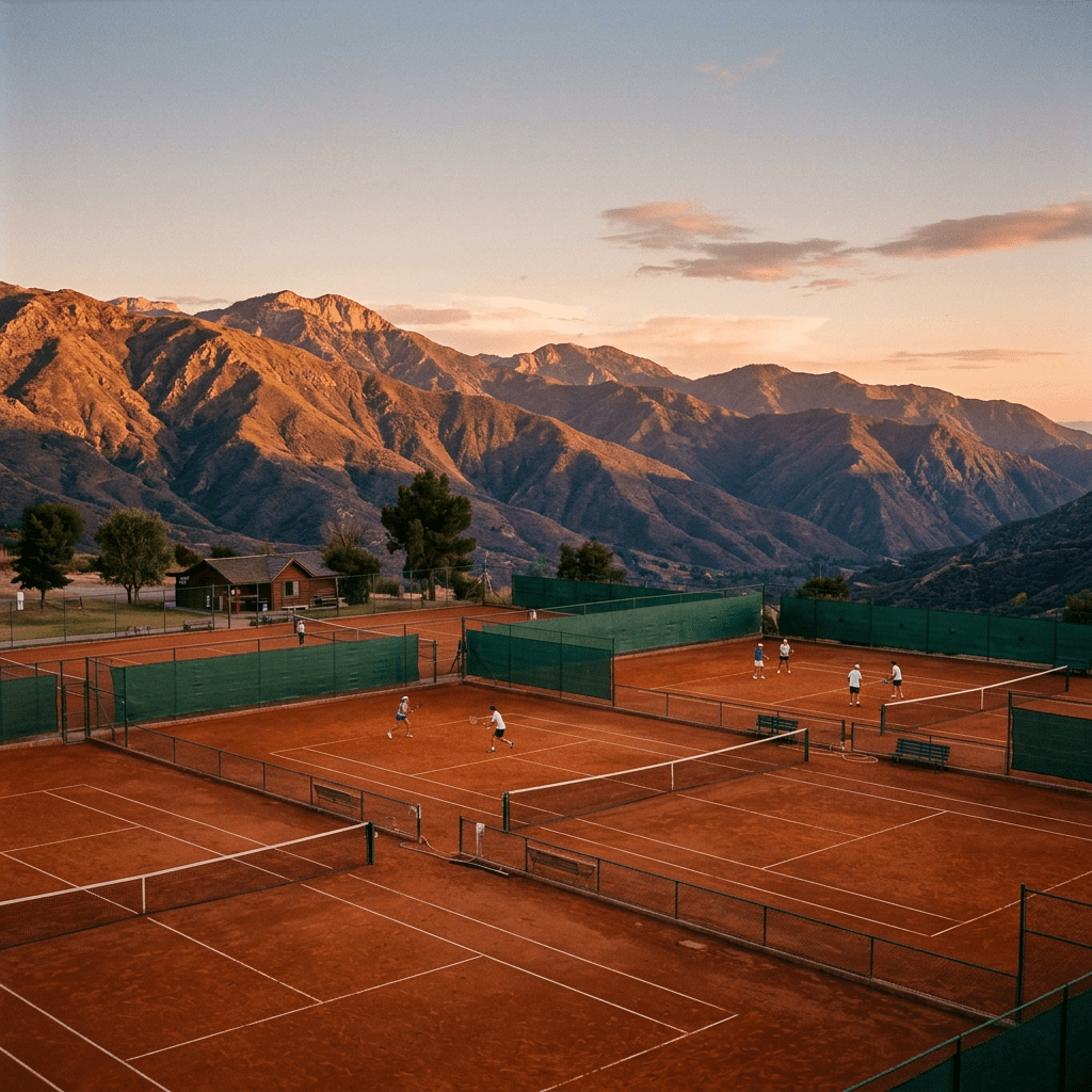
Their players grow up inside systems built around constant competition.

The Hidden Advantage

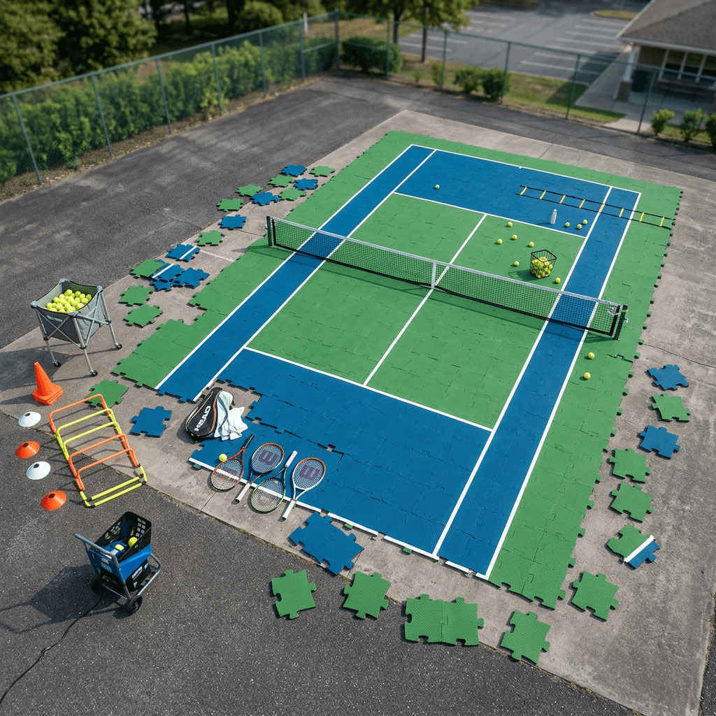
In 2026, Spain will host 31 Futures tournaments (Futures are the lowest rung of professional tennis, where players earn their first ATP points). Italy will host 23.

Similarly, just from the beginning of 2026 until the end of July – so seven months – Spain will host 9 Challenger events (the level just below the ATP Tour events most people see on TV), and Italy will host 14(!!).

Canada is nowhere near that level. As of right now, there are 3 Futures tournament scheduled in 2026, and 3 Challengers between now and July.

The exact number of tournaments might change a little from year to year, but the difference is massive.

And that difference changes development.

A player based in Spain or Italy can lose the first round one week, drive a few hours, and compete again next week, often on the same surface.

That creates a completely different developmental environment than what most Canadian players experience.

Competing professionally becomes normal instead of exceptional.

In Spain or Italy, a young player may personally know dozens of others trying to make it professionally. Futures and Challengers are not some distant level you occasionally hear about. They are part of the local tennis ecosystem.

In Canada, most aspiring pros probably know only a handful of players attempting that path seriously.

Why This Matters So Much

A lot of improvement in tennis does not happen in practice. Matches force players to solve problems, regulate emotions, figure out tactical adjustments, and manage pressure. Those things develop fastest through repetition in real competitive environments.

Not through another controlled practice set.

Real competition exposes weaknesses quickly. And when players compete every week, they get faster feedback loops.

Europe Allows Players to Stay Inside the System

One of the biggest advantages in Spain and Italy is not just tournament quantity. It is the ability to stay inside the ecosystem consistently, and simply continue competing.

A player can build long stretches of competition with:

minimal flights
lower travel costs
less disruption to training
familiar surfaces and conditions

For example, Martin Landaluce played his first pro event in October 2022. Between October 2022 and January 1st, 2024, he played 29 events. Out of those 29, 19 were in Spain. A few others were in Portugal or France, neighbouring countries. He was able to get from being unranked, to #450 ATP, while not having to travel prohibitively, control his expenses, and compete in clubs he’s probably been to a few times before.

A Canadian player often has to spend heavily just to access enough professional-level matches: flights, hotels, rental cars, coaching expenses (if those are even realistic), and weeks away from home.

Eventually, every tournament starts feeling financially important. Every loss matters a little more. That changes development too.

The Canadian Challenge

Canada has absolutely produced world-class players. Milos Raonic, Denis Shapovalov and Félix Auger-Aliassime proved that.

The issue is not talent, or inferior coaching. The issue is density. There are simply fewer opportunities for Canadian players to compete regularly, build ranking points gradually, and develop through volume of meaningful matches.

Canadian players often have to become international much earlier in their careers. That creates higher costs, more logistical stress, less continuity, and more pressure attached to results.

And for many players, that pressure arrives before they are fully ready for it.

Why Competitive Density Helps Late Developers

Dense competition ecosystems allow players more time; not every player is physically or mentally ready to turn pro at 18.

If college tennis maybe isn’t an option, but when there are constant professional opportunities nearby, players can survive longer while continuing to improve.

In thinner systems, players often disappear earlier because the economics and logistics become unsustainable. Some late bloomers are just players who were given the time to mature, find their game, and survived long enough to develop.

Final Thought

I do not think the success of Italian and Spanish tennis is just about coaching quality or talent identification.

Those countries have built ecosystems where competition is:

accessible
frequent
sustainable

And over time, that compounds. Players improve fastest when competition becomes part of normal life instead of an expensive event that happens occasionally. That may be one of the biggest advantages in modern player development.

The Real Problem With Most Tennis Programs (No One Is Responsible)

Portable tennis court mat with net, tennis balls, rackets, and training cones

Most tennis academies and private clubs aren’t built around player development.

They’re built around volume.

More players in programs
More group sessions
More private lessons

From a business standpoint, that makes sense. More of everything drives revenue growth, keeps the courts busy, and maintains the impression of an engaged member base.

From a development standpoint, the individual player can get lost in the shuffle. That’s because in a lot of the clubs, no one actually owns the development of the player.

Everyone Is Involved. No One Is Responsible.

A typical competitive junior schedule can look like this:

2–3 different group sessions per week, maybe even at different facilities
Private lessons with one or two different coaches
1-2 fitness sessions on the side

On paper, it looks like a lot of work is being done.

But is all of that work pointing in the same direction?

Each coach is running their own session.
Each session has its own focus.
The fitness and tennis coaches might not even know each other.

The player ends up with:

Different messages
Different priorities
No clear direction

It’s not that the coaches aren’t good.

It’s that the system isn’t connected.

Group Training Isn’t the Problem—But It Has Limits

Group sessions are efficient. But they are, by design, generalized. The themes and drills need to be applicable to everyone in the group.

They’re not built around:

One player’s patterns
One player’s weaknesses
One player’s competition schedule

So unless something is built around them, the player just becomes part of the group.

They get better in a general sense, and a hit a large volume of balls.

But their actual development becomes… vague.

Private Lessons Don’t Fix It

Parents often try to solve this by adding private lessons.

That seems logical:

“More individual attention should solve the problem.”

But if those lessons are with different coaches, and there’s no shared plan, it just adds more noise.

Now the player is getting:

Slightly different technical cues
Slightly different tactical ideas
No consistent framework

Fragmentation instead of clarity.

The Missing Link: Communication

In a well-functioning development environment:

Tennis coaches talk to each other
Fitness coaches know the physiological demands of tennis
Competition schedules influence training
There’s a clear progression

In most environments, that doesn’t happen.

Fitness is done separately. Tennis is done separately. Competition and tournaments happen on weekends, with the club coaches rarely present, and post-match analysis skipped over (if done at all) rather than take as a guide to the next few sessions of practice.

No one is tying it together.

So Who Ends Up Managing It?

The parents.

They’re the ones trying to:

Piece together a schedule
Decide which coach to listen to
Figure out what tournaments to play
Understand what their child actually needs

All while:

Working full-time
Being a parent first
Not being experts in player development

It’s an impossible role.

And yet, in most systems, it’s the default.

What This Leads To

Over time, you start to see patterns:

Players training a lot but not improving in a clear direction
Confusion around identity (“What kind of player am I?”)
Gaps between practice and competition
Burnout—from doing a lot without a clear purpose

From the outside, it looks like the player just “stalled.”

In reality, the environment never gave them a coherent path.

What’s Missing Isn’t More Training

Most of these players don’t need:

More hours
More clinics
More lessons

They need:

A plan.

Not a vague idea.

A clear, communicated, evolving plan that answers:

Who am I on a tennis court? What are my strengths and weaknesses?
What am I trying to achieve tactically?
Do I have the physical, technical, and competitive tools to execute my tactical goals under pressure?
If not, what is the roadmap to achieve those tools?

And most importantly:

Someone with a map and a 30,000 ft view responsible for it.

A Better Model (That Rarely Exists)

At a minimum, every serious player should have:

One person who oversees development
Alignment between coaches
Integration between tennis, fitness, and competition
Clear communication with the player and parent

It doesn’t have to be complicated.

But it has to be intentional.

Final Thought

Most academies and clubs aren’t doing anything “wrong.”

They’re just optimized for something different.

They’re optimized to run programs—not to manage individual development.

And those are not the same thing.

Until someone takes ownership of the player’s path, progress will always depend more on luck than design.

And that’s a hard way to build a player.

Why Most Tennis Players Plateau (And It’s Not What You Think)

Tennis player kneeling on court holding head in frustration near racket

Ask most players why they’ve plateaued and you’ll get some version of:

“I need to work harder”
“My technique isn’t there yet”
“I just need more reps”

That sounds logical.

It’s also the reason they stay stuck.

Most players don’t plateau because of effort. And they don’t plateau because their forehand needs another 5,000 balls.

They plateau because they’re not actually training the skill that decides matches:

Decision-making.

The Practice Looks Good. That’s the Problem.

Watch a typical session.

Balls are being fed. The player is moving well. Contact is clean. Rhythm is there.

If you walked by, you’d think: this is solid training.

But look closer.

The ball is predictable
The situation is predictable
The decision is often made in advance (or doesn’t exist at all)

The player isn’t solving anything.

They’re executing in a controlled environment.

That can look good for a long time without actually improving performance.

Matches Are a Different Game

Then they go play a match.

Now:

The ball isn’t predictable
The opponent is changing things constantly
Time disappears
Pressure shows up

And suddenly the same player looks “inconsistent.”

But most of what we call inconsistency isn’t technical.

It’s decision quality breaking down under pressure.

Wrong target. Wrong timing. Wrong pattern.

That shows up as missed shots—but the miss isn’t the root problem.

More Reps Just Dig the Hole Deeper

The default fix is always the same:

“I just need more reps.”

So players go back and hit more balls in the same environment that caused the problem.

Now they’re just getting better at executing without making decisions.

That doesn’t transfer.

You can hit a clean forehand all day in practice and still choose the wrong shot 20 times in a match.

At some point, it’s not about how well you can hit.

It’s about whether you’re choosing the right thing to hit.

The Skill That Actually Separates Players

At higher levels, it’s rarely about who has better strokes.

It’s about who:

Recognizes situations faster
Chooses higher-percentage options
Adjusts patterns based on what’s happening

That’s not technique.

That’s awareness + decision-making.

And most players barely train it.

What Needs to Change

If your practice doesn’t force decisions, it’s limited.

That doesn’t mean feeding is useless. It just means it’s incomplete.

At some point, the player has to:

Read something
Decide something
Live with the outcome

That’s where improvement actually happens.

Simple examples:

Don’t just rally—add constraints on when you can change direction
Don’t start every drill neutral—start in disadvantage or attack situations
Don’t measure reps—pay attention to decisions

Now you’re training something that exists in matches.

Plateaus Aren’t Random

If you’ve been at the same level for a while, it’s not bad luck.

It’s your training environment doing exactly what it’s designed to do.

It’s building a certain level of player—and then stopping.

More volume won’t fix that.

Better design will.

A Better Question

Instead of asking:

“How do I hit this better?”

Ask:

“What’s the right decision here—and can I recognize it fast enough?”

That’s a different level of problem.

And it’s the one that actually moves players forward.

Final Thought

Most players aren’t that far off.

They just spend too much time in practice that doesn’t look like the game.

Tennis isn’t just execution. It’s problem-solving under pressure.

If you don’t train that, you shouldn’t expect it to show up when it matters.

Second Serves: The Need for Speed

As players progress in their tennis careers, arguably the hardest transition they go through is jumping from high level junior tennis to the professional ranks. The world of fancy hotels, top notch facilities, and feeling of proximity to the top of our sport is replaced by the reality of Futures – the minor leagues of professional tennis. You need to climb the rankings ladder again by competing in remote tennis clubs, where time on the practice court often constitutes wishful thinking, and for the first time you’re playing against opponents literally fighting for their livelihood.

Besides needing to adjust to this new reality mentally and emotionally, I often get asked what the main differences are in the actual game, on-court, between high level junior and high level professional players. One area is the speed of the game, and I’d like to illustrate this point using second serve speed data from the men’s and boys’ draws from this year’s Wimbledon.

Below is a table that has the average second serve speeds from the boys’ draw on the left, and the men’s draw on the right. I looked at the round of 16 onwards in both cases, for 30 total data points each.

Juniors: Avg 2nd Serve Speed (mph)	Round	Men: Avg 2nd Serve Speed (mph)	Round
91	R16	104	R16
103	R16	106	R16
92	R16	107	R16
100	R16	104	R16
98	R16	97	R16
103	R16	97	R16
96	R16	100	R16
91	R16	99	R16
97	R16	103	R16
100	R16	98	R16
95	R16	101	R16
101	R16	98	R16
91	R16	106	R16
93	R16	91	R16
97	R16	97	R16
98	R16	104	R16
97	QF	104	QF
96	QF	110	QF
104	QF	100	QF
93	QF	101	QF
103	QF	106	QF
100	QF	103	QF
88	QF	96	QF
88	QF	107	QF
97	SF	110	SF
104	SF	105	SF
99	SF	107	SF
91	SF	106	SF
95	F	108	F
91	F	105	F

96.4	Mean	102.67
22.52	Variance	20.99

Data Courtesy of Wimbledon.com

Without going too deep into statistics, we would use something called an unpaired t-test to determine whether the difference in means between the two groups is statistically significant. In our particular case – we have 30 observation in each category, with the means and variances listed above – we get a p-value of less than 0.0001. We can conclude, with a high degree of certainty (in our case more than 99.999%) that we do have a statistically significant result. In our case, in layman’s terms, we can be fairly certain that the top pros hit their second serves at a higher speed than the top juniors.

I would argue that there are three components that go into an effective second serve:

Speed
Placement/depth
Variety

All three play a role in keeping the opponent off-balance, and starting the point at a roughly equal footing. A greater speed gives a greater margin for error; all else equal, I’d rather miss my spot with a 100-mph second serve than with a 85-mph one.

The sample that I used has obvious limitations: I didn’t look at first serves, I didn’t look at the whole draw, and I only considered one tournament, on grass. But I think that it still illustrates, or at least suggests, that the speed of the game is different between the pro game and the juniors. If I was coaching a junior with professional tennis aspirations right now, getting his average second serve speed in the neighbourhood of 100mph would certainly be one of the metrics on my list.

Does Success at Les Petits As Predict Success in the Pros?

Les Petits As is widely considered as one of the most important junior tennis tournaments in the world. Held in Tarbes, France, it is the unofficial world indoor championship in the Under-14 category. The list of singles winners, on the men’s side, includes well-known legends of our sport such as Rafael Nadal, Richard Gasquet, or Juan Carlos Ferrero. But rather than relying on just a couple of names, I wanted to take a wider view, and see, whether success at Les Petits As can serve as a predictor of success on the professional level.

Before going over the findings, there are a couple of choices I had to make that limit the number of players I considered. First, I decided to only look at the singles draws of Les Petits As, and the career high ATP singles rankings of the athletes in question. Second, I have defined success at Les Petits As as making the quarter-finals or better. This would give me 8 players per year, and with looking at 11 historic draws (years 2007-2017), 88 players total. A good enough sample size, but not overwhelming to do in an afternoon. Finally, I defined success on the professional tour as making the ATP Top 100 or better.

In short, is making the quarter-final of Les Petits As a sure-fire predictor of future professional success? It is not. Out of the 85 unique players – Francis Tiafoe, Borna Coric, and Nikolay Vylegzhanin made the quarter-final or better twice – 16 have made the ATP Top 100 as of April 14th, 2025. Here is the full list:

Name	Nationality	LPA Result	Year of Result	Career High ATP Rank
Holger Rune	DEN	SF	2017	4
Luca Nardi	ITA	W	2017	67
Hamad Medjedovic	SRB	F	2017	71
Chun Hsin Tseng	TPE	W	2015	83
Miomir Kecmanovic	SRB	F	2013	27
Alex De Minaur	AUS	QF	2013	6
Alexei Popyrin	AUS	QF	2013	23
Francis Tiafoe	USA	W	2012	10
Mikael Ymer	SWE	QF	2012	50
Michael Mmoh	USA	SF	2012	81
Hubert Hurkacz	POL	QF	2011	6
Alexander Zverev	GER	SF	2011	2
Quentin Halys	FRA	W	2010	54
Borna Coric	CRO	SF	2010	12
Liam Broady	GBR	F	2008	93
Jiri Vesely	CZE	QF	2007	35

16 out of 85 is a success rate of less than 20%. There are a few players, especially from the more recent editions of Les Petits As, who might still crack the Top 100; Harold Mayot, for example, who made the semifinals of the 2016 edition of Les Petits As, has a career high of 103. But the overall picture stays the same. If you pick a player at random, and all you know about him is that he made the quarter-finals of Les Petits As, there is a less than 1 in 5 chance that he’ll make it to the Top 100, based on this particular set of data.

In fact, picking a random quarter-finalist from the 11 editions of Les Petits As from 2007-2017, you’d be almost as likely to find someone, who didn’t earn an ATP ranking at all, as you would a future Top 100 player. 14 out of the 85 players have not achieved an ATP ranking in their career as of yet.

Finally, if we assign a ranking value of 0 to the players, who have not earned an ATP ranking, the median career best ranking for the 85 players is #215; roughly speaking a challenger-level player.

What is there to learn from the above exercise? If a player reaches the quarter-finals, or better, at Les Petits As, he will most likely earn at ATP ranking. But the likelihood of that player cracking the Top 100 is about 1 in 5. It’s a long and winding road to the top, even in tennis. Even the best 14 year olds are just at the start of their journey.

The Predictable Carlos Alcaraz

One of the things that makes watching Carlos Alcaraz play tennis so exciting is the variety in his game. When his feet are set for a forehand, he is equally adept at blasting a 100mph missile, or use his touch and send a soft drop shot barely over the net. He can slice, come to the net, lob, defend exceptionally well..there are not many holes to exploit in his game. However, during his 2025 Australian Open quarter final defeat at the hands of Novak Djokovic, he was too predictable on one particular shot. And in a match decided by a few points, that proved too costly.

Here are the serving statistics from their match; Djokovic on the left hand side, Alcaraz on the right.

Alcaraz had the upper hand when the first serve was put in play, winning 67% of those points compared to 63% for Djokovic. But Alcaraz couldn’t get anything going behind his second serve, winning only 33% of the points, well below the 58% of Djokovic. Djokovic is one of the best returners in the history of our sport, but Alcaraz’ predictable second serve placement helped him out last night.

Here is where Novak Djokovic aimed his second serves against Alcaraz:

In the deuce side, Djokovic served wide on 48% of his second serves, 24% into the body, and 28% into the Alcaraz backhand. In the ad side, the breakdown was 31%/46%/23%. The lowest overall percentage is 23% – out wide in the ad side. That is still almost one out of every four second serves in the ad side, and forces the returner to cover the whole box.

By contrast, here is the second serve placement map for Alcaraz:

In the deuce court, Djokovic could have eliminated the wide third of the box completely when getting ready to receive Alcaraz’ second serve. In the ad side, only 9% of Alcaraz’ second serves went down the T, into the Djokovic forehand.

By completely avoiding the Djokovic forehand return, Alcaraz gives Djokovic an invitation to set up the point however he likes. Djokovic can either step in, and take his backhand return early – made easier by the fact that he can wait in his backhand grip and give up a third of the box. Or, he can back up to get a forehand return anyway – here he can start moving early, while Alcaraz’ ball toss is still in the air, because he knows that the serve will be aimed toward a particular area of the box.

Alcaraz has made some changes to his serve technique before the Australian Open already. He is one of the most electric players on tour, and the scary thought is that, at such a young age, he still has room to improve. Mixing up his second serve placement, making it more unpredictable, would complement the rest of his game, and help even out the second serve battleground in his next encounter with Novak Djokovic.

Not a Fan of Dirt

Clay is certainly not Daniil Medvedev’s favorite surface, and he’ll happily tell you so. Despite winning the Masters 1000 in Rome this year, Medvedev’s preferred surface is hard. He’s won his only Grand Slam title on the hard courts of US Open in 2021, made the finals in New York in 2019, as well as making the finals at the 2021 and 2022 Australian Open championships.

After making the finals of the 2023 ATP 1000 in Indian Wells, and taking home the title in Miami, Medvedev lost in the quarter finals of Monte Carlo to Holger Rune, and in the round of 16 in Madrid to Aslan Karatsev. Before going on to win the title in Rome, he stated that he wanted to focus on more spin and better sliding on clay.

Without watching the matches, it is impossible to judge whether Medvedev looked more comfortable sliding. I did, however, wanted to check whether there was any significant difference in the spin rates of Medvedev’s groundstrokes on the hard courts as opposed to the clay courts.

In order to do that, I looked at Medvedev’s forehand and backhand spin rates in Indian Wells and Miami this year (hard court events), and compared them to the spin rates of his groundstrokes from Monte Carlo, Madrid, and Rome (clay court events). I ended up having 10 data points for the hard courts, and 12 data points for the clay courts. To test for statistical significance, I used the unpaired t test for both the forehands and backhands, with a 95% confidence interval.

Forehands

	FH Hard Courts	FH Clay Courts
Mean	2,361.60 rpm	2,297.92 rpm
St. Deviation	98.20 rpm	161.47 rpm
Sample Size	10	12
p-value	0.2894

Data courtesy of ATPTour.com

On the forehand side, there was no significant difference in the spin rates of that stroke on the hard courts and the clays. Overall, Medvedev’s forehand was the “spinniest” during his R32 match against Ilya Ivashka in the R32 match in Indian Wells, where it averaged 2,511 rpm. On the other hand, it was the “flattest” in his R32 match on the clay courts of Madrid against Alexander Shevchenko, with a 1,992 rpm average.

Backhands

	BH Hard Courts	BH Clay Courts
Mean	1,486.10 rpm	1,387.25 rpm
St. Deviation	107.15 rpm	77.21 rpm
Sample Size	10	12
p-value	0.0207

Data courtesy of ATPTour.com

On the backhand side, there is a statistically significant difference between the two data sets, but it is in the opposite direction that Medvedev intended. In these particular samples, his backhand ended up being flatter on the clay courts than on the hards.

Medvedev is not known for using a lot of slice backhands at all, so I doubt that the difference in spin rates on the backhand side would be due to him hitting more slices on the hards or the clays. Adding more spin to a stroke would usually involve a change to the grip or the racket path of a stroke (or both). Backhand is arguably one of Medvedev’s biggest weapons, and maybe he wasn’t comfortable changing any of those variables to generate more spin.

It’s hard to say whether Medvedev’s flat backhand is one of the reasons for his relative clay court struggles. He hits one of the flattest backhands on the tour, and on the hard courts his stroke will stay low after the bounce, making an aggressive response from the opponent challenging. On clay courts however, the backhand will bounce a little higher, closer to the preferred strike zone of the opponent around his waist, making it easier to attack. In the end, regardless how Medvedev planned on adding more spin to his groundstrokes, his strategy didn’t work this year. With the grass court and hard court swings yet to come, Medvedev can at least look forward to his favorite part of the year.

Beneath The Surface Of Tennis

When trying to forecast the outcomes of our decisions, one of the more widely used mental models differentiates between first-order and second-order consequences. First-order consequences are the more obvious, surface-level ones. They also tend occur relatively early after the decision is made. Understanding second-order consequences requires a deeper analysis, looking beyond the obvious. Second-order consequences also tend to manifest themselves after a certain period of time has elapsed following the decision has been made.

For example, let’s say a tennis player decides to skip a warm-up at the beginning of a training session. Through a first-order lens, this might be a positive; the player has an extra 10 or 15 minutes to work on her strokes. But through a second-order lens, the skipped warm-up looks more like a negative; the player increases her chances of injury, is not physically prepared for the first few drills of the session, and might learn to place a lesser importance on her physical preparation overall.

A few examples of first-order thinking in the tennis world that have recently caught my eye are:

Don’t work on overheads, you never hit them in matches. This statement is true on the surface. In matches, we hit way more groundstrokes, serves, and returns than we do overheads. Practice time is limited, so why waste it on a stroke that we might hit once a set. If we look a bit deeper though, we realize that a player who doesn’t spend any time on her overheads will not be confident in that stroke. As a result, that player won’t be comfortable coming to the net during the matches. Spending time on the overhead, even though it is a relatively infrequently hit shot, is an important aspect of developing attacking tennis players with a well-rounded game.

Focus only on singles. When playing tournaments, doubles can often be an afterthought. After all, the majority of practice time is traditionally spent on singles, and very few juniors initially aspire to be outstanding doubles players. When looking a bit deeper though, if doubles is not taken seriously, we miss out on an opportunity to work on serves and returns – the two most important strokes in tennis – in a match situation. We don’t take advantage of thinking through movement, angles, and positioning in a different way than in singles. Finally, we don’t learn how to win and lose as a team, and how to communicate with our partner – all skills that extend beyond the tennis court.

Only practice with players better than you. Initially, that seems to make sense. When training with somebody who is better than us – hits the ball harder, is in better shape, can exploit our weaknesses effectively – we can clearly see which areas of our game need improvement. In a group setting, if we are one of the weaker players, it forces us to focus harder and push ourselves more than if we were one of the stronger players. Upon a deeper examination though, playing with weaker players has a lot of positives too. We can adjust our game style to work on things that are outside of our comfort zone. For example, serve and volley once a game. Play only through the middle. Tell yourself that you’re not allowed to hit winners and instead outlast your opponent. Play with only one serve. Start every game at 0-30. There are countless ways how to make practice productive when we are the stronger player.

I’m sure there are a lot of other examples of first and second order thinking in tennis. If you think of some good ones, leave them in the comments!

Nick Kyrgios The Tactician

It would be an understatement to say that Nick Kyrgios is a polarizing figure in the world of professional tennis. He is a Grand Slam champion, and one of the most talented athletes in our sport. At the same time, one can never be quite sure what is going to happen when watching one of his matches. Will we see a brilliant performance, worthy of a Top 10 player? Will we see indifference, broken rackets, and arguments with the chair umpire? One is as likely as the other.

In the second round of the Miami Open, we got to see the former. Kyrgios demolished Andrey Rublev, currently ranked #7 in the world, in 52 minutes by the score of 6-3 6-0. During the course of the match, we caught a glimpse of a side of Nick Kyrgios that doesn’t get spoken about very often: Kyrgios the tactician, executing a game plan to perfection.

Going into the match, Kyrgios knew that “…he’s (Rublev) a player who relies on a bit of rhythm, so I just tried to keep the points short and sharp, just play aggressive.” I want to highlight one way that Kyrgios set himself up to do just that.

If there is a knock on Rublev’s game, it is that his second serve is relatively slow. Below is a chart comparing the average serve speeds between Kyrgios and Rublev from their match:

Average Serve Speed	Nick Kyrgios	Andrey Rublev	Difference
1st serve	207 km/h	193.6 km/h	13.4 km/h
2nd serve	171.9 km/h	143.8 km/h	28.1 km/h

Courtesy ATPTour.com

Attacking Rublev’s second serve would be a great starting point to keep the rallies short and putting immediate pressure on the Russian. And Kyrgios did just that, with his positioning and impact point. This is the average return position of Kyrgios in the match when returning Rublev’s second serve:

Two meters inside the baseline is about as aggressive as you can be with hitting the return on the rise and taking time away from the opponent. The beauty of this return strategy – when looking at it through the lens of Kyrgios’ overall tactic of keeping the points short – is that there is very little downside. If you hit a quality return, great! You’re most likely ahead in the rally, as there is a high chance that Rublev is rushed and off-balance on the first groundstroke after the serve. If you miss the return – the rally length was 1, and Rublev doesn’t get a chance to get into any sort of rhythm.

The strategy worked beautifully. Rublev won only 4 out of the 19 points played on his second serve (that’s 21%; generally speaking, we would like the server to be around the 50% range). Furthermore, almost three quarters of all points contested in the match were played in the 0-4 rally range:

Rally Length	Kyrgios Won	Rublev Won	Total	% of Total
0-4	42	23	65	73%
5-8	9	7	16	18%
9+	2	6	8	9%

Courtesy ATPTour.com

Just for comparison, here is Kyrgios’ second serve return position in his third round match against Fabio Fognini. He still returned from inside the baseline, but he toned down the aggressiveness:

In the round of 16 match, Kyrgios is set to face Jannik Sinner. I would assume that Kyrgios won’t be looking to engage in prolonged baseline exchanges in that match either. His second serve return positioning will give you a hint as to the quality of Sinner’s second serve, as well as the style of match that Kyrgios will want this to be.

Carlos Alcaraz and Second Serve Placement

After the conclusion of the 2022 Australian Open, all the talk on the men’s side – and rightfully so – has been about Rafael Nadal and his 21st Grand Slam title. As much as Nadal has meant to the sport, it is no secret that the proverbial clock is ticking, and he is at the very tail end of his magnificent career. As one of the legends of tennis nears retirement, Spanish tennis has another young superstar waiting in the wings. I would never put the label of “heir apparent” to Nadal on anyone; Nadal’s achievements are unique and unmatched. But Carlos Alcaraz might be the next Spanish player to sit on the throne of men’s professional tennis.

Alcaraz is 18 years old, and ranked #29 in the world as of January 31st, 2022. If you haven’t seen him play, he is far from your typical Spanish clay court specialist. His is a complete attacking game, with the power to dial up a first serve in the 130mph range, control the rallies with his massive forehand, but also transition to the net and hit the occasional drop shot . The scary thing for the rest of the professional tennis world is that at 18 years of age, Alcaraz can only get better. And one area, where Alcaraz can elevate his game, is his 2nd serve placement.

Let’s use Alcaraz’ 3rd round match at the Australian Open against Matteo Berrettini as an example. A cursory look at the surface statistics doesn’t raise any red flags: Alcaraz won an exceptional 61% of his second serve points (anything over 50% is considered a good day in the office). Could this number have been even higher? This is the placement of all of Alcaraz’ 2nd serves from the match:

On both sides of the court, Berrettini could have eliminated a third of the service box when he was receiving Alcaraz’ second serve. Alcaraz hit 51 second serves in the match, and only two of them were directed at Berrettini’s forehand. On the one hand, the tactic was working – as demonstrated by the 61% second serve winning percentage. On the other hand, it will free Berrettini to do something like this (at the 1 minute 46 second mark):

Berrettini breaks Alcaraz in the first game of the second set by forcing an error behind an aggressive inside-in forehand. What allowed Berrettini to set his feet and really unload on that forehand was the depth and quality of his backhand return. If Berrettini knows that Alcaraz will not serve his forehand in that situation, he can either run around the second serve to start the rally with a forehand return, or – like he did here – step inside the court, wait for the serve with a backhand grip, pick a return target before Alcaraz even hits the serve, and get on offense right away.

Was this maybe just a tactic against Berrettini? Is Alcaraz more unpredictable with his second serve location in other matches? Here is the placement of his second serves from this 2nd round match against Dusan Lajovic:

Even in this match, Alcaraz served exclusively into the backhand and body of Lajovic. Alcaraz ended up winning this match rather easily in three sets, but even then the location of his second serves, from both sides of the court, was predictable.

How can a player get more comfortable with hitting a particular area of the service box with his second serve? The first step, as it usually does, happens in practice. You could play a practice set where you’re only allowed to hit second serves out wide in the deuce side, and down the T in the ad side. The second step would include hitting the second serve to that area in matches, in low leverage situations. For example, if you’re up 40-0 in a game, go for the second serve down the T. Even if you lose the point, you’re still heavily favored to win the game, serving at 40-15. Alcaraz won the first two sets against Lajovic 6-1 6-2. Firmly in control of the match, he still didn’t hit any second serves to the Lajovic forehand in the third set. Finally, the third step is hitting that serve in matches, in high leverage situations: tie-breaks, when facing break points etc.

For Carlos Alcaraz, the sky is the limit. He is one of my favorite players to watch and will be the face of men’s professional tennis for years to come. He already plays with an aggressive mentality from the baseline; harnessing that same mindset with his second serve locations should not be too difficult of a task.